Mass flow rate, ![]() , is the mass of fluid passing through a boundary per unit of time. It is defined as:
, is the mass of fluid passing through a boundary per unit of time. It is defined as:

where ![]() is the fluid density, v is the fluid velocity integrated over the boundary, S.
is the fluid density, v is the fluid velocity integrated over the boundary, S.
The mass flow rate through a boundary can be easily measured experimentally using a mass flow meter. Mass flow meters have replaced other forms of flow rate measurement because of their accuracy, precision, and resolution of flow measurement. Coriolis, inertial and thermal mass flow meters are available.
Because of the ease of measurement, the mass flow rate is typically the physical quantity known. Hence, when simulating a system, the mass flow rate is the input boundary condition prescribed in the simulation model. Such systems include hydraulic manifolds, pumps, compressors, jets, and biomechanical systems such as cardiovascular systems, amongst many others.
For incompressible flow problems with fixed boundaries, the mass flow rate through a boundary can be prescribed using the velocity boundary condition. However, for compressible flow problems, or for fluid-structure interaction (FSI) problems with deforming boundaries, the velocity for a given flow rate is a function of the fluid temperature, pressure and boundary deformation, which are not known a priori.
In ADINA CFD and ADINA FSI, the mass flow rate through a boundary can now be directly prescribed using the mass flow rate boundary condition.
When the mass flow rate boundary condition is applied to a boundary, the ADINA CFD/FSI solver automatically creates a reasonable velocity profile across the boundary that closely represents the fully-developed velocity profile. For example, for a circular boundary, a Poiseuille-based velocity profile is applied, as shown in Figure 1. This velocity profile is then used to compute the fluid solution variables in the solution domain. During each fluid-solution iteration, the velocity magnitude on that boundary is adjusted such that the prescribed mass flow rate is maintained.
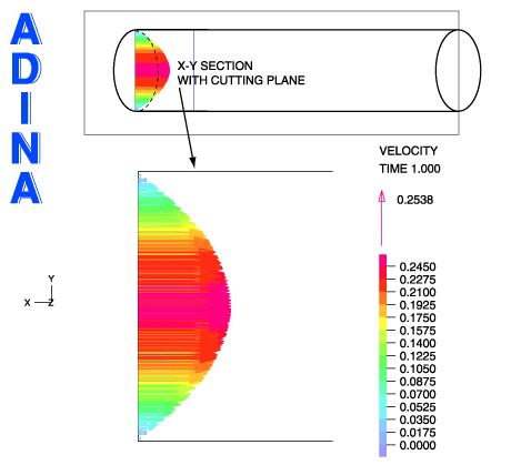 Figure 1 Velocity profile applied to a circular boundary by the mass flow rate boundary condition
The flow direction applied by the mass flow rate boundary condition can be specified. There are three options:
- Normal Inflow: The flow direction is normal to the boundary and the fluid flows into the fluid domain.
- Normal Outflow: The flow direction is normal to the boundary and the fluid flows out of the fluid domain.
- Vector: The flow direction is specified by the user-input direction vector.
The user can further adjust the flow direction applied by the mass flow rate boundary condition to follow the geometry of the neighboring boundaries, as shown in Figure 2.
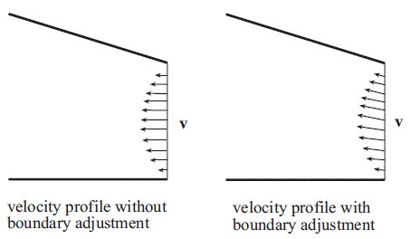 Figure 2 Velocity profile applied by the mass flow rate boundary condition with boundary adjustment with boundary adjustment; the flow direction changes smoothly from the bottom horizontal direction to the upper inclined boundary direction
The mass flow rate boundary condition offered in ADINA CFD/FSI can also be used to prescribe a volume flow rate through a boundary. Volume flow rate, ![]() , is the volume of fluid passing through a boundary per unit of time. It is defined as:
, is the volume of fluid passing through a boundary per unit of time. It is defined as:

where v is the fluid velocity integrated over the boundary, S.
Prescribing a volume flow rate through a boundary can be useful for fluid-structure interaction problems that have deforming boundaries.
Illustrative Examples
We give some illustrative examples to demonstrate the mass flow rate boundary condition. We consider the following three problems:
- 2D-axisymmetric model of incompressible flow through a pipe with a moving FSI boundary.
- 3D model of compressible flow through a pipe with time-dependent temperature.
- 3D model of an artery FSI simulation.
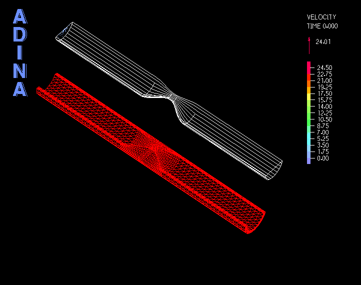
In the first example, we show a 2D-axisymmetric model of incompressible flow through a pipe with a moving FSI boundary, see Figure 3, and as a consequence the pipe inlet is changing in size. A constant mass flow rate is prescribed to the inlet using the mass flow rate boundary condition.
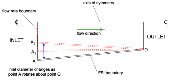 Figure 3 2D-axisymmetric model of incompressible flow through a pipe with a moving FSI boundary
The movie in Figure 4 shows the velocity solution. We see that the mass flow rate boundary condition automatically computes a reasonable fully-developed velocity profile at the inlet, and adjusts the velocity magnitude to maintain a constant mass flow rate.
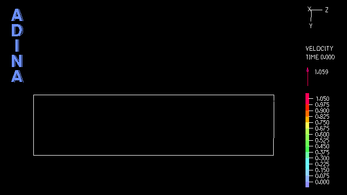 Figure 4 Velocity solution for the 2D-axisymmetric model of incompressible flow through a pipe with a moving FSI boundary
Next, we show a 3D model of compressible flow through a pipe with a time-dependent temperature. A constant mass flow rate is prescribed to the inlet using the mass flow rate boundary condition, see Figure 5.
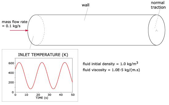 Figure 5 3D model of compressible flow through a pipe with a time-dependent temperature profile
The movie in Figure 6 shows the velocity solution. We see that as the temperature varies, the density of the fluid varies, and the mass flow rate boundary condition automatically varies the velocity magnitude at the inlet to maintain a constant mass flow rate.
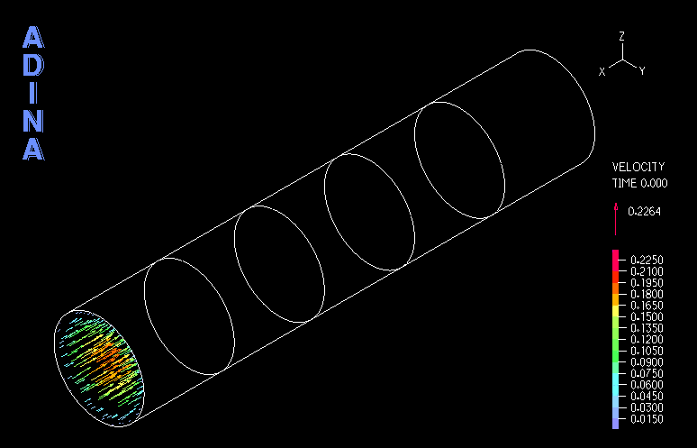 Figure 6 Velocity solution for the 3D model of compressible flow through a pipe with a time-dependent temperature profile
–In the final example, we show a 3D fluid-structure interaction model of an artery simulation with stretching, see Figure 7. A constant mass flow rate is prescribed to the inlet of the artery using the mass flow rate boundary condition. A prescribed displacement is applied to the solid model to stretch the artery. Arteries are flexible muscular tubes lined with tissue. Large deformations in the artery and the constant mass flow rate result in large velocity variation along the artery, especially the non-uniform inlet velocity profile, and hence this is a highly-nonlinear fluid-structure interaction problem.
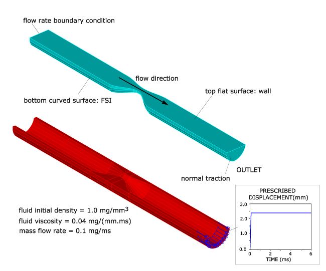 Figure 7 3D model of an artery FSI simulation; fluid model (top) and structure model with prescibed displacement boundary condition (bottom).
The movie at the top of this Tech Brief shows the artery deformation. Figure 8 shows that as the artery deforms, the mass flow rate boundary condition automatically varies the velocity magnitude at the inlet to maintain a constant mass flow rate.
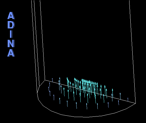 Figure 8 Velocity solution at the inlet of the 3D artery FSI simulation
Summary
The mass flow rate boundary condition is a powerful feature in ADINA CFD/FSI to prescribe the mass flow rate or volume flow rate through a boundary for compressible flow problems, and for fluid-structure interaction problems where the boundary deforms during the solution.
Keywords:
Mass flow rate, volume flow rate, compressible flow, fluid-structure interaction, artery simulation