Using L-Systems in GenerativeComponents

L-Systems or Lindenmayer Systems is a mathematical formalism developed by biologist Aristid Lindenmayer in 1968 to mimic plant growth. Later, its application was further extended in computer graphics for creating self-similar structures and generating plant models. 

In this post, we will see how we can use L-Systems in GenerativeComponents to create different types of geometries. 

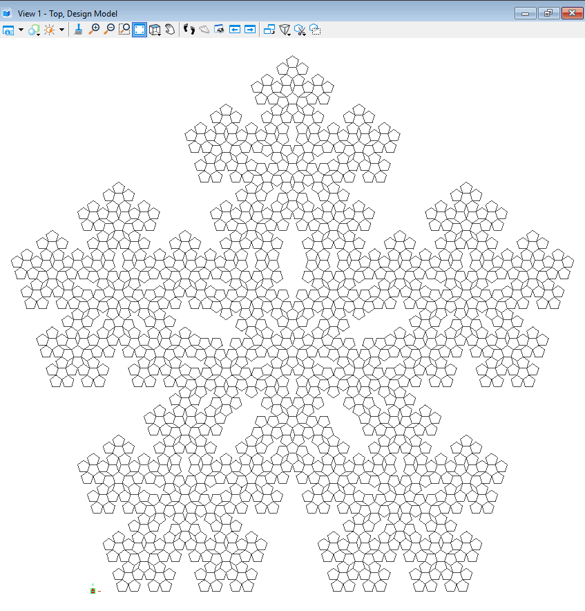
An illustration of a geometry created using L-Systems in GC

How do L-Systems work?

In L-System, the key concept revolves around how to rewrite an initial element in each successive step based on certain rules in order to get the final structure. 
The most basic type is called DOL i.e., Deterministic, Context free L-System. Let’s understand with the following example

To begin with, let us consider ‘B’ to be the initiator. This initiator is called axiom. Then, the rule of rewriting for the successive steps will be, B->A, A->BA  

Rewriting in each generation as per the rule

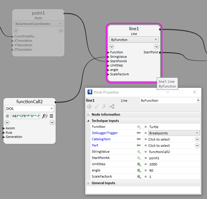
‘DOL’ in GC

When there is any term for which there are no rules, it will pass to the next generations. For the purpose of these DOL we have a function called ‘DOL’ in GC. 
The input for Axiom is string type, e.g., ‘A’ or ‘FFA’ 

The input for rule is table type, e.g., we will write the above rule in the following form:
{[‘B’] = ‘A’, [‘A’] = ‘AB’} 

This function is called inside a FunctionCall node.

Turtle Interpretation of the DOL Output

Once we have the string output from the DOL function, we need to create the required geometry from it. This geometric interpretation approach is, indeed, inspired from the popular ‘Turtle’ programming language. For this reason, in this approach, each character of the DOL output act a command for the function Turtle.  
Let’s further understand this by looking at an example and the commonly followed syntaxes:

To begin with, let us imagine the Turtle as a moving coordinate system. The turtle, then, moves forward if it encounters command ‘F’ and turns left or right by a given angle if it encounters ‘+’ and ‘-‘.  

Thus, with string input ‘FF-F+F’:

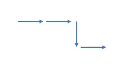
Drawing in turtle as per input ‘FF-F+F’ 

Commands of Turtle

'F' to move forward by drawing a line i.e in X-direction of local Coordinate System 
'f' move without drawing anything  i.e in X-direction of local Coordinate System 
'+' turn left by given angle about local Z axis 
'-' turn right by given angle about local Z axis 
'&' Pitch down by given angle or rotate in anticlockwise direction about local Y-axis 
'^' Pitch up by given angle or rotate in clockwise direction about local Y-axis 
'/' Roll left by given angle or rotate in anticlockwise direction about local X-axis 
'' Roll left by given angle or rotate in anticlockwise direction about local X-axis 
'|' Turn 180 about local Z-axis 
'>' Scale up unit length  
'<' Scale down unit length 
'[' Save current Coordinate System information, location, scaling factor 
']' Move to last saved Coordinate System information, location, scaling factor

The Axiom and Rule of DOL is chiefly set keeping the above turtle commands in mind.

The Turtle Function in GC can, in essence, perform all the above. However, for this, it takes only 5 inputs: 

1. String Value, i.e., the turtle command or the DOL output 
2. Start Point, i.e., Starting point of the turtle. The coordinate system of this point will be the first coordinate system of turtle. 
3. UnitStep, i.e., The distance by which Turtle moves forward at each step. 
4. Angle, i.e., The angle by which the turtle turns based on the command. 
5. Scaling Factor, i.e., The factor by which UnitStep is scaled up or scaled down based on the command. When not required use value 1 
   
   

A Simple Example of L-System

Let us, further, take a look into a simple example. For this purpose, we will see how to construct Koch curve using L-System.

Firstly, it starts with a single line in X-direction Axiom: ‘F’ 

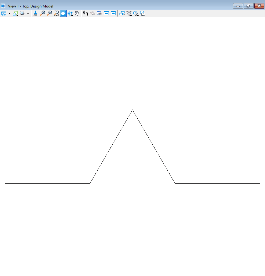
Once the single line is created, at every subsequent generation, each line will be converted into a set of 4 lines. These 4 lines are a result of the following rule:

{[‘F’] = ‘F+F–F+F’}. 
Angle =  60 

Generation 1

Generation 1

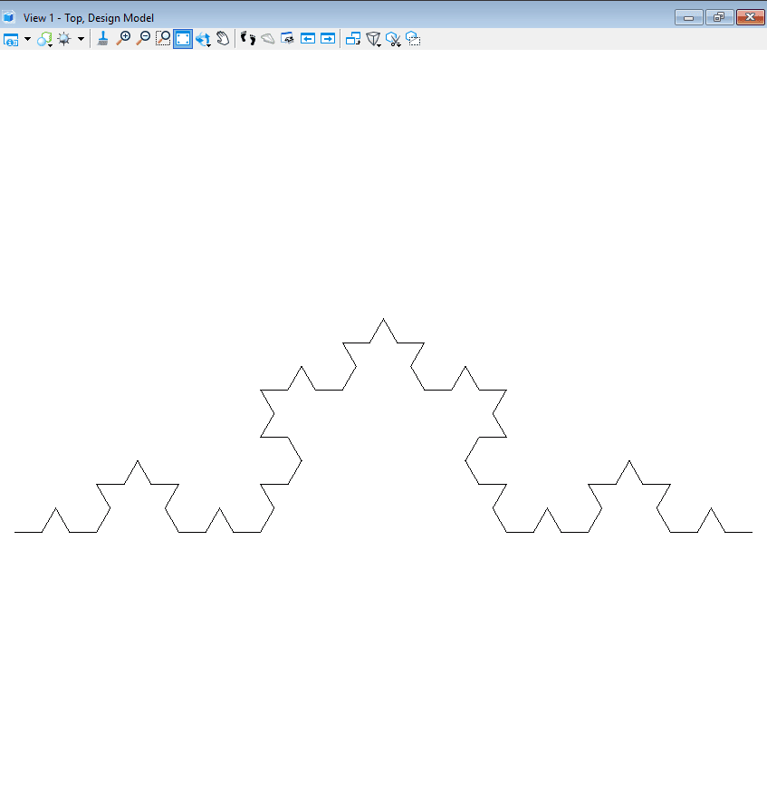
Generation 2

Generation 3

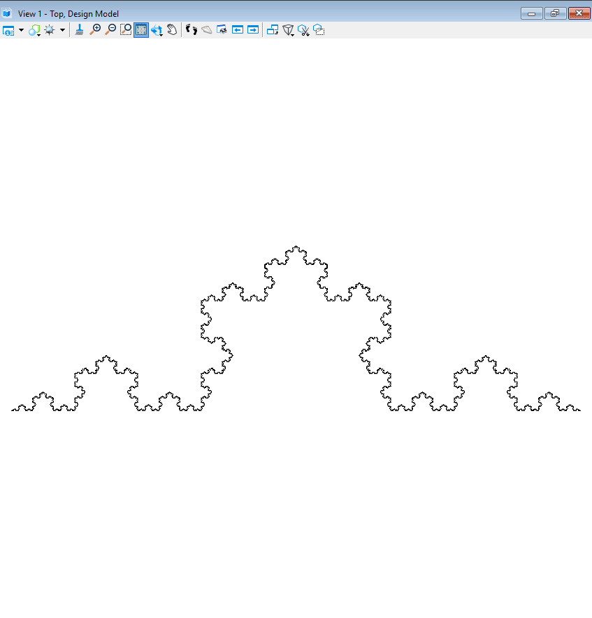
Generation 6

Further, Examples of L-Systems

Combination of Island and Lake

Axiom: ‘F+F+F+F’ 
Rule:{[‘F’] =  ‘F+f-FF+F+FF+Ff+FF-f+FF-F-FF-Ff-FFF’, [‘f’] = ‘ffffff’} 
Angle 90 
Generation: 2 
Scale Factor = 1 

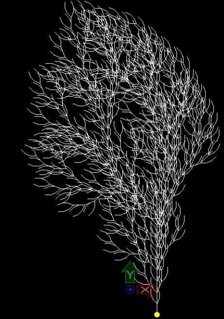
Stick Tree

Axiom = ‘++a’
{[‘F’] = ‘>F<‘, [‘a’] = ‘F[+x]Fb’, [‘b’] = ‘F[-y]Fa’, [‘x’] = ‘a’, [‘y’] = ‘b’}
Angle = 45
Generation:12
Scale Factor = 1.36

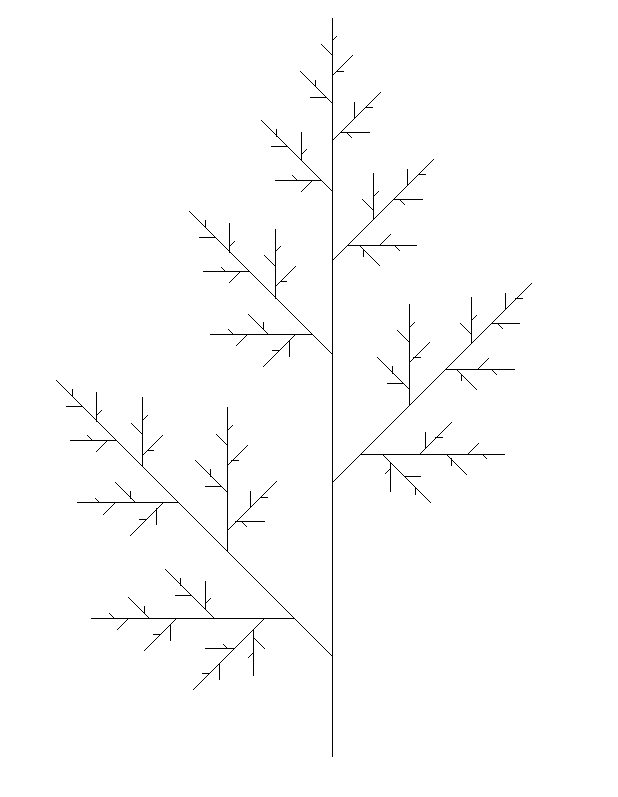
2D Bush Tree

Axiom: ‘F’
Rule: {[‘F’]=’FF+[+F-F-F]-[-F+F+F]’}
Angle: 22.5
Generation: 4
Scale Factor: 1

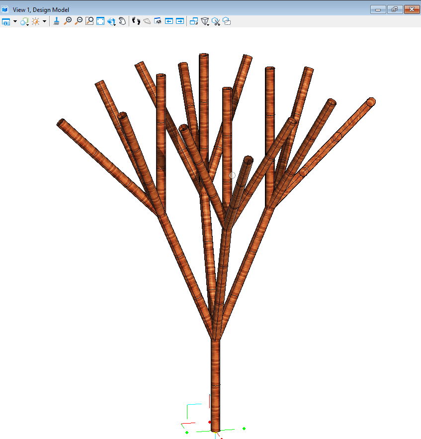
Simple 3D Tree

Axiom: ‘^^^^FFA’
Angles: 22.5 º
Rules: {[‘A’]= “[B]////[B]////[B]////B”,  ‘[‘B’] = ‘&FFFA’}
Generation: 3
Scale Factor: 1

Once we get the line, we can use that to create a Bspline surface around it using the SweepCircleAroundPath technique.

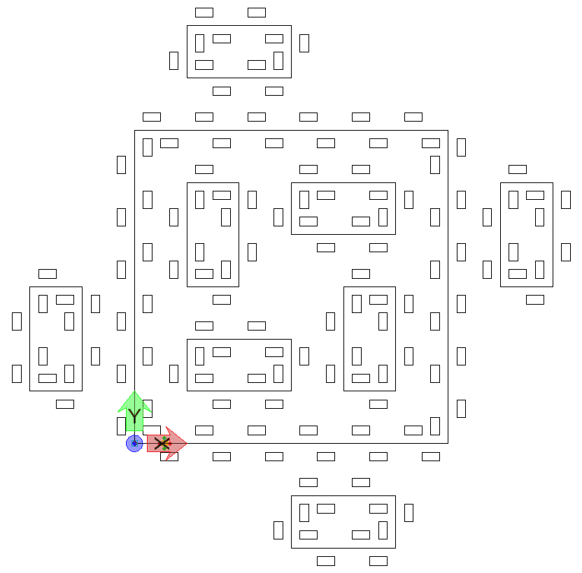
3D Hilbert Curve

Axiom: ‘A’
Rule:  {[‘A’] = ‘B-F+CFC+F-D&F^D-F+&&CFC+F+B//’, [‘B’] = ‘A&F^CFB^F^D^^-F-D^|F^B|FC^F^A//’ , [‘C’] = ‘|D^|F^B-F+C^F^A&&FA&F^C+F+B^F^D//’, [‘D’] = ‘|CFB-F+B|FA&F^A&&FB-F+B|FC//’}
Generation: 2
Angle: 90
Scale Factor: 1

Furthermore, for more examples you can go here. As a matter of fact, some of the above examples are actually adopted from there.

Further Scope of Work

1. Include turtle command to create close polygons
2. Stochastic context free L-system where rules will be selected stochastically.

Reference and Further Reading

Prusinkiewicz P, Lindenmayer A (1990). The Algorithmic Beauty of Plants. Springer-Verlag: New York

You can also find good resources here.