How to Set Up the Fluidity Parameter γ of the Hoek-Brown Model with the Softening Model
In the framework of numerical analyses of geomaterials, one of the classical problems for modeling the development of shear bands is the pathological mesh-dependence of the computed solution which implies failure without energy dissipation. To avoid this unphysical behavior, an internal length must be introduced to govern the evolution of the shear band thickness in the post-peak regime of the material response.
More specifically, it is well known that introducing too large a difference between the dilatancy angle
 and the equivalent friction angle
 will lead to a mesh-dependent solution which then will be almost systematically associated with:
- Numerical convergence difficulties, and
- Potentially convergence toward an incorrect solution.
The numerical solution then becomes ill-posed and the conditioning of the numerical solution further worsen as the difference between the dilatancy angle and the friction angle increases or as the element size in which shear bands develop as a result of shear failure becomes smaller.
In this context, the Hoek-Brown with softening (HBS) model uniquely proposes a feature to restore the mesh-objectivity of the numerical solution through a visco-plastic regularization based on the over-stress theory of Perzyna, thus enabling the introduction of an internal length through a temporal gradient. The use of the viscous regularization technique in the Hoek-Brown model with softening is a definite advantage when one wants to consider a high level of non-associativity and maintained mesh-objective solution as shear plastic strains further develop.
This modeling technique requires the introduction of:
- A loading rate which is created by associating a physical time duration in the calculation phase this technique is introduced.
- An extra model parameter called the fluidity γ (which is the inverse of a viscosity) that needs to be properly calibrated in relation to the previously introduced rate of loading.
The idea is to simulate a circular tunnel excavation in an infinite Hoek-Brown medium subjected to an in-situ isotropic stress field
![]()
Using a given set of HBS model parameters, this simple excavation analysis will be run multiple times, with each time a different value for the fluidity γ (all other model parameters remaining constant, of course). Once all runs are terminated, the radial stress evolution over the radius can be plotted and the influence of the fluidity parameter in terms of stress development can be properly evaluated and quantified.
Most specifically, we are interested in the computation of the stress evolution over the plastic radius surrounding the excavated area. The plastic radius can be evaluated from the closed form solution provided by Carranza-Torres and Fairhurst (1999).
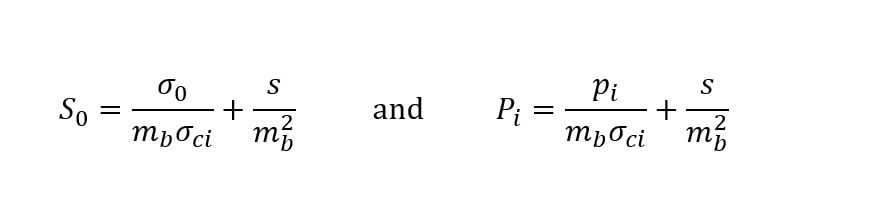
The scaled far-field stresses, S0, and scaled internal pressure, Pi, are determined by:
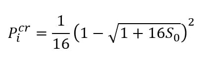
Then the scaled critical internal pressure, , at which the elastic limit of the stress state is reached, can be calculated as:
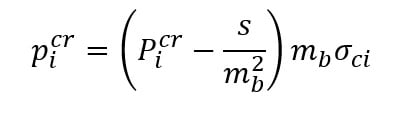
The critical internal pressure, , is then:
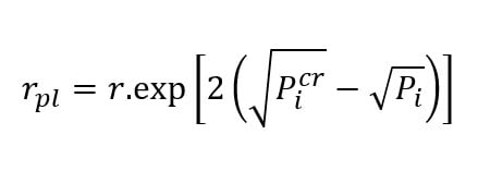
A plastic region developing uniformly around the hole will develop only if is larger than the supporting pressure. The extent of the failure zone is:
Setting Up the PLAXIS Model
The PLAXIS model created will be an axisymmetric model corresponding to a very thin slice of the cylindrical hole in the rock mass (see Figure 1). A thickness of 0.1 m is perfectly sufficient, the idea being to have a calculation that runs as quickly as possible. The tunnel will be placed vertically, but as the initial stresses will be set by the stress field feature, there will be no need for gravity forces to be accounted for during initial stress definition and unit weight for the rock mass could be set to 0. A circular tunnel of radius r will be then be excavated with an applied supporting pressure pi.
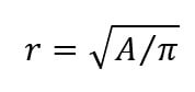
The radius r corresponds to the equivalent radius of the considered tunnel cross section (which might not necessarily be circular). In that case, if A is the excavated area of the real tunnel, then:
R has to be sufficiently large to avoid boundary effects. For instance, R = 5 rpl could be accounted for.
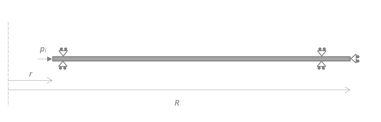
Figure 1: Model geometry of axisymmetric tunnel analysis.
Project properties will define the model contour ranging from xmin = 0 to xmax = R. For the vertical model extent, one can define ymin = -0.1 to ymax = 0.
One soil borehole containing a single layer ranging from 0 down to -0.1 m could then be introduced. Place the water level at an arbitrary low level to ensure the soil formation will remain dry (for instance, Head = -1 m).
Soil material properties are defined using the user-defined soil model HB-GSM or HB-SSM contained in the hbs64.dll. The drainage type will be Drained. It is important to set both saturated and unsaturated unit weight to zero as previously explained. Model parameters should then be defined by the user. Note that each fluidity value that the user is willing to investigate should lead to the definition of a new material set (such that there are as many material sets as fluidity values to be considered).
In the Structures mode, it is important to partition the geometry and introduce geometry lines at:
- x = r for the definition of the excavated area.
- x = rpl to facilitate the post-processing and make clear the consideration of the plastic zone in PLAXIS output.
Boundary conditions are defined by prescribing fixed vertical direction over the bottom and top horizontal lines and fixed horizontal displacement at x = R. A distributed load should also be applied at x = r to represent the (optional) supporting pressure (see Figure 2a).
The mesh should be generated by making sure that there will be just one element in the thickness direction (y-axis) for the model run to perform as quickly as possible (see Figure 2b).
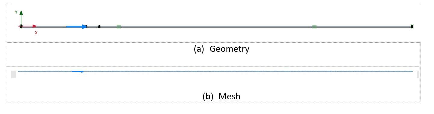
Figure 2: PLAXIS 2D Model Presentation
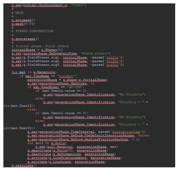
In the calculation mode, initial stresses are defined during the initial phase by means of field stress with a uniform state of stress σ1 = σ2 = σ3 = -σ0. Then, as many plastic analyses should be independently created (from the initial phase) as there are fluidity parameters (and, therefore, independent material sets) to be investigated (see Figure 1). For each calculation phase, it is important to:
- Deactivate the excavated soil cluster,
- Deactivate default boundary conditions from the model explorer (model conditions → deformations),
- Activate for each calculation phase the prescribed displacement along with the distributed load if non-zero.
It is also very important to associate to each calculation phase a duration Δt = 10 days that will define the rate of loading. Ultimately, the loading rate effect will solely be a function of γ´Δt. Still, we prefer to give to Δt a reasonable physical meaning, although it would not be necessarily required, as finally γ´Δt = (10γ) ´ (Δt/10)!
Finally, by setting to just 1 the maximum number of cores to be used for each phase (numerical control parameters -> max core to use), then independent calculation phases could be run simultaneously, resulting in an even shorter overall calculation time.
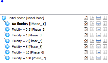
Figure 3: Phase Definition
Once the calculation has terminated, one can enter PLAXIS Output, only displaying the plastic area cluster (by hiding the other soil cluster from x = rpl to x = R) and visualize the Cartesian Total Stress σxx (radial stress) as shown in Figure 4.
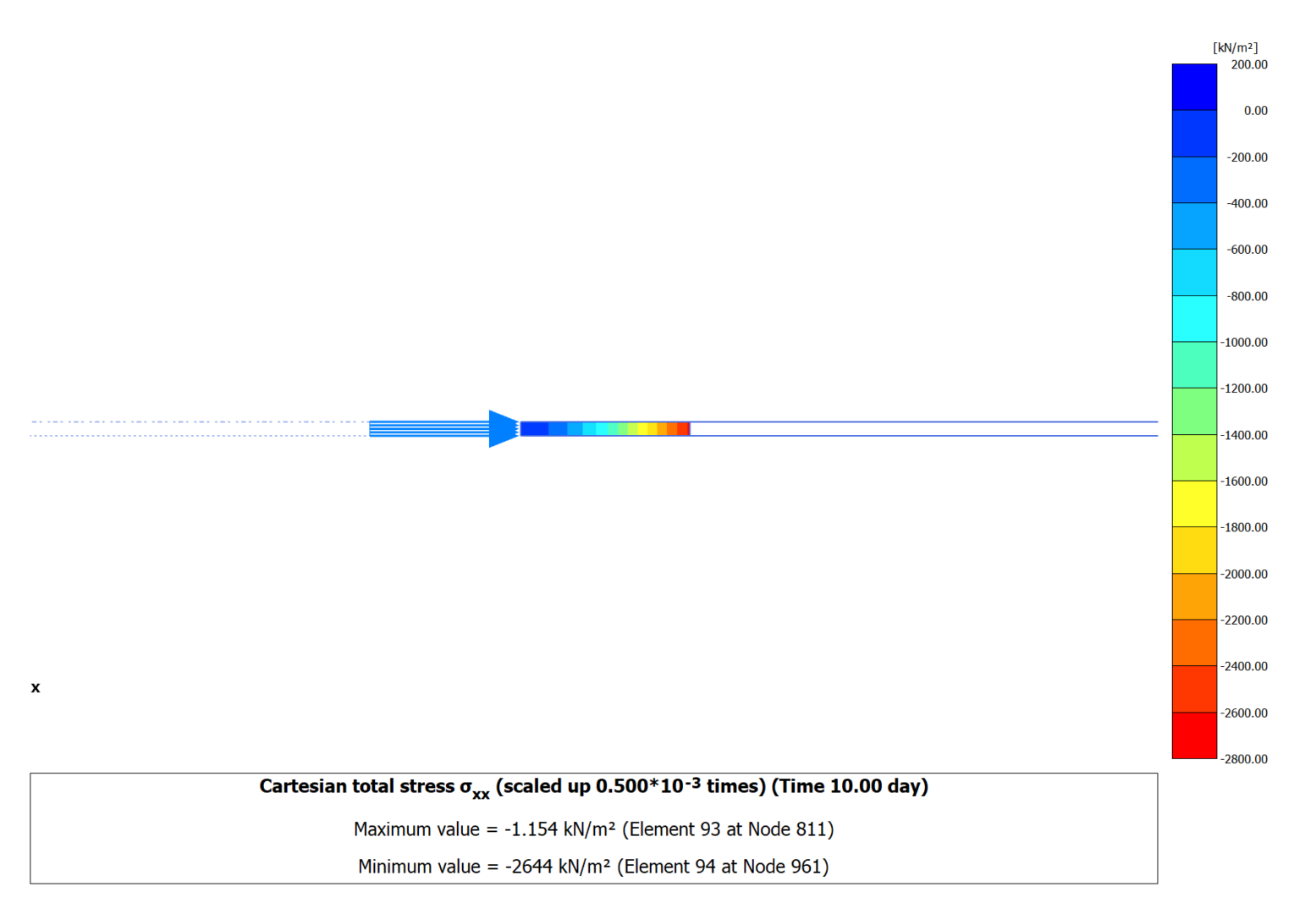
Figure 4: Contour plots of Cartesian total radial stress
Then one can draw a cross section from x = r to x = rpl and then apply the cross section tool that will require the selection of the last steps of each plastic calculation phase (as shown in Figure 5).
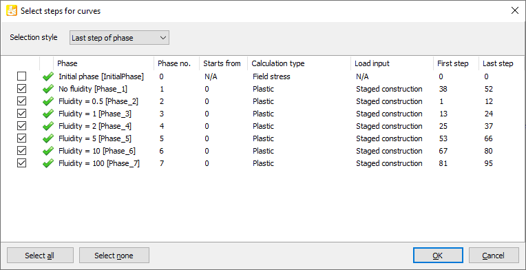
Figure 5: Step selection for curves
Results obtained in this context are displayed in Figure 6.
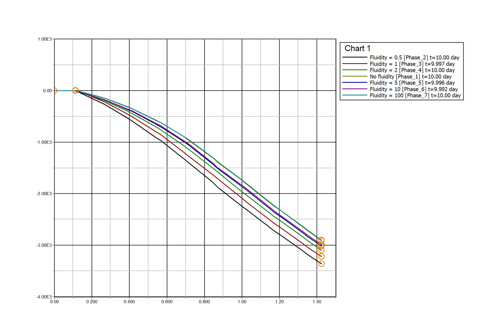
Figure 6: Radial stress evolution in the plastic zone as a function of the fluidity parameter γ.
Automation and Python Scripting
The process documented in the previous section has been fully automated in a Python script called fluidityVariationStudy.py. All functions being called are presented in the Appendix.
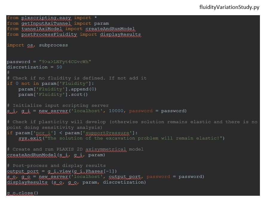
What the script basically does is exactly the same as what has been presented in the previous section. It finally displays the radial stress evolution through the plastic zone as a function of the fluidity parameter γ. Additionally, it computes the relative area under the stress-radius curves to quantify the difference between each fluidity parameters value (see Figure 6).
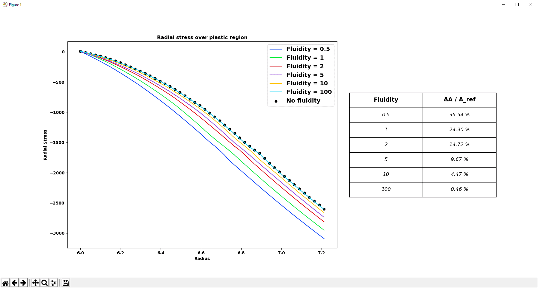
Figure 6: Automated presentation of the radial stress evolution in the plastic zone as a function of the fluidity parameter γ.
References
Carranza-Torres, C., and Fairhurst, C. (1999). “The elasto-plastic response of underground excavations in rock masses that satisfy the Hoek-Brown failure criterion” – International Journal of Rock Mechanics and Mining Sciences, 36(6), 777-809
Appendix
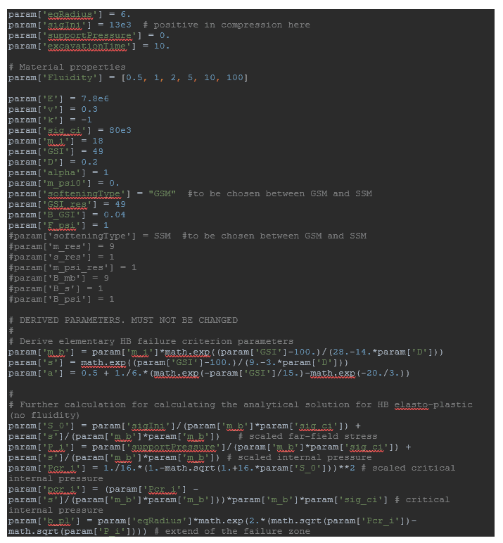
The input parameters are summarized in a dictionary param being defined by the user in getInputAxiTunnel.py.
The createAndRunModel function constructs the PLAXIS 2D calculation model based on the user-defined set of parameters and runs the calculation. It can be found in tunnelAxiModel.py.
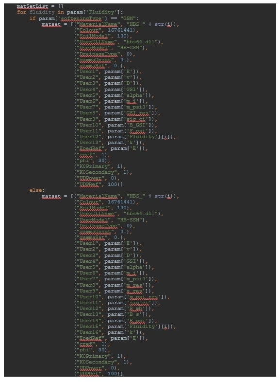
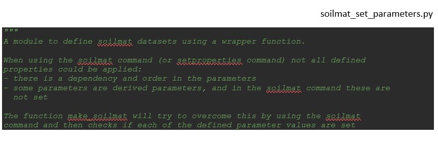
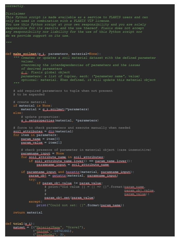
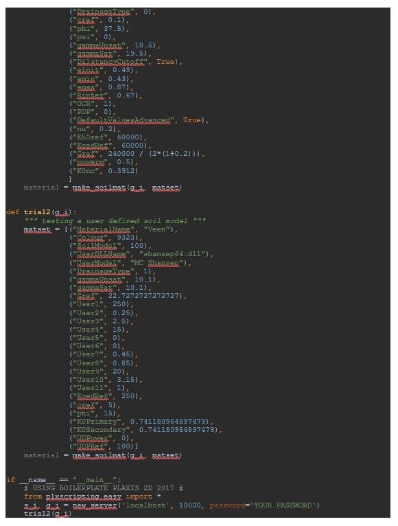
The material sets are created based on a special function called make_soilmat to be found in soilmat_set_parameters.py.
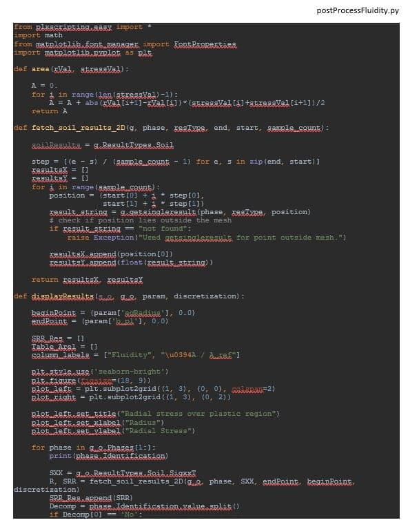
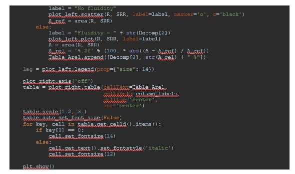
Finally, post-processing functions are defined in postProcessFluidity.py.