On the launch of ADINA version 9.4 (ADINA 9.4) one year ago, it was announced that the new ADINA sparse solver released in ADINA 9.4 achieves considerable speedups with no compromise in accuracy. This speed increase is of great value to industry — in particular, the automotive, aerospace, defense, industrial equipment, heavy machinery, civil, and consumer product industries — that frequently need to run large, high-fidelity simulations.
Over the past year, we have heard from our ADINA customers that the new ADINA sparse solver has significantly increased their productivity, while maintaining a high level of accuracy, giving them a significant advantage.
In this Tech Brief, we will show some examples of the performance of the new ADINA sparse solver released in version 9.4. We show representative test models and actual customer models. The models are solved using ADINA 9.3 and ADINA 9.5, and the solution times and memory usage are compared.
All models except no. 4 have been solved using an Intel Xeon E5-2667 v4 workstation with 16-cores and SMP (no DMP). Model no. 4 was solved using an Intel Xeon CPU E5-2687W workstation with 16-cores and SMP (no DMP).
Models
This section describes the models considered.
Model 1 – Linear static analysis
- 3D block meshed using 8-node 3D-solid elements.
- Pressure loading applied to the top surface. Fixities applied to all degrees of freedom (DOF) on the bottom surface.
- Linear static analysis, 1-time step.
- Total number of DOFs = 1,952,802
Figure 1 Model 1 – Finite element mesh for linear static analysis of a 3D block
Model 2 – Nonlinear contact analysis
- Two 3D blocks in contact meshed using 8-node 3D-solid elements.
- Pressure applied to the top surface of the top block. Fixities applied to all degrees of freedom (DOF) applied on the bottom surface of the bottom block.
- Nonlinear contact analysis, 1-time step.
- Total number of DOFs = 2,850,246
Figure 2 Model 2 – Finite element mesh for nonlinear contact analysis of 3D blocks
Model 3 – Nonlinear contact analysis
- Ring bearing model meshed using 8-node 3D-solid elements.
- Nonlinear contact analysis, 5-time steps.
- Total number of DOFs = 3,119,969
 Figure 3a Model 3 – Finite element mesh for nonlinear contact analysis of a ring bearing
 Figure 3b Model 3 – Animation of effective stress results
Model 4 – Frequency analysis of a six-cylinder engine block
- Meshed with 10-node tetrahedron 3D-solid elements.
- Besides the sparse solver improvement, the Enriched Bathe Subspace Iteration method is used in 9.5 compared to the Standard Bathe Subspace Iteration method for 9.3;
200 frequencies and mode shapes are calculated. - Total number of DOFs = 9,494,250
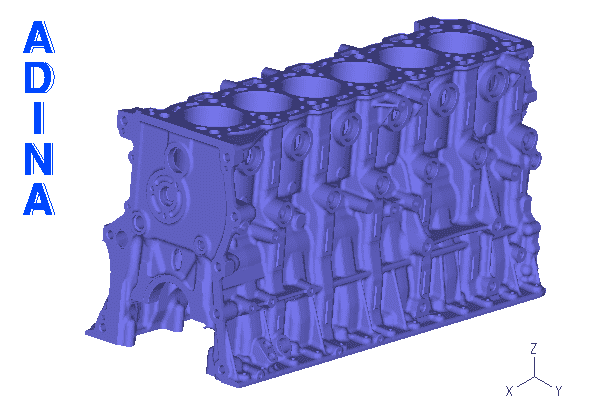 Figure 4a Model 4 – Finite element mesh for frequency analysis with contact of a six-cylinder engine block
Figure 4b Model 4 – Animation of mode shape 1
Model 5 – FSI analysis
- Hydraulic engine mount
- Direct-coupling FSI, 21-time steps. Fluid model: 8-node elements, Solid model: 20-node elements
- Total number of DOFs = 852,672
Figure 5a Model 5 – Fluid finite element mesh for FSI analysis of a hydraulic engine mount
Figure 5b Model 5 – Animation of deformation with effective stresses and fluid velocity vectors
Solution time and memory usage results
The solution speedup is defined as:
The memory usage reduction is defined as:
![]()
Table 1 compares the total solution times of ADINA 9.3 and ADINA 9.5.
Table 1 Total solution times for ADINA 9.3 and ADINA 9.5
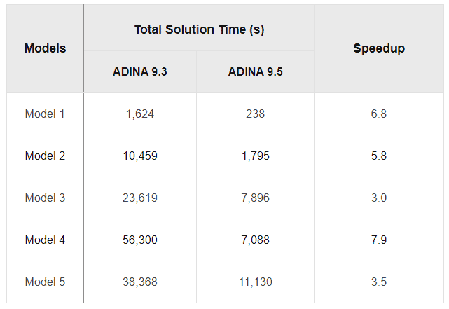
Table 2 compares the memory usage of ADINA 9.3 and ADINA 9.5.
Table 2 Memory usage of ADINA 9.3 and ADINA 9.5
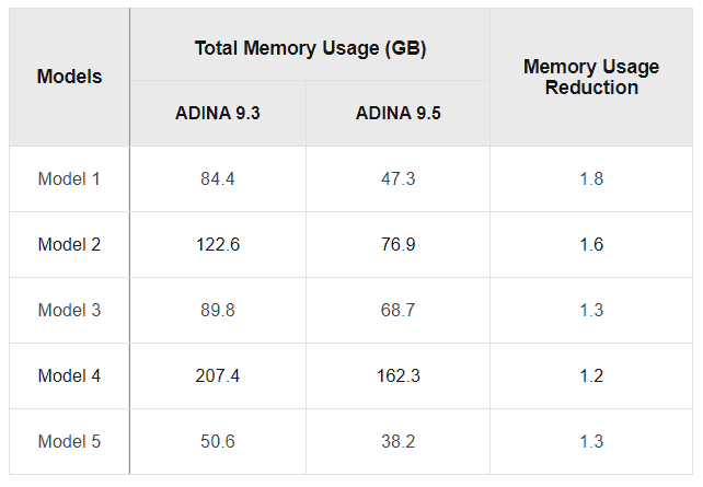
Tables 1 and 2 show that the new ADINA sparse solver released in version 9.4 achieves considerable speedups and memory usage reductions for a wide range of applications, including linear, nonlinear, contact, frequency, and FSI analyses.
For the models considered in this Tech Brief, the new ADINA sparse solver is 3 to 7 times faster than the sparse solver in ADINA 9.3.
SMP parallel-processing performance results
The SMP performance rate is defined as:
![]()
Table 3 summarizes the SMP performance rates of ADINA 9.5 for Model 1.
Table 3 SMP performance rates of ADINA 9.5 for Model 1
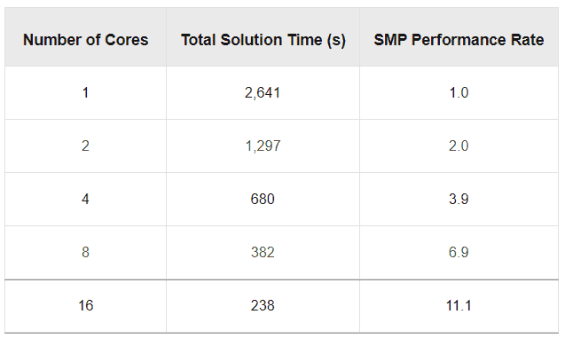
The table shows that the ADINA sparse solver released in version 9.4 achieves good SMP scalability as the number of cores is increased.
Conclusions
The new ADINA sparse solver released in version 9.4 clearly greatly strengthens the ADINA System allowing customers to increase their productivity, while maintaining a high level of accuracy, for a wide range of analysis problems.
Keywords:
Sparse solver, frequency analysis, contact analysis, efficiency, improvement, productivity