
I occasionally hear people say they use a second-order equation to model chlorine decay when in a perfect world, chlorine decay should follow a first-order model. I wondered why that worked.
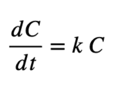
As a matter of review for those who haven’t studied much chemistry lately, the general equation for most chlorine decay models is:
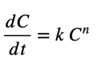
Where C = concentration, k = reaction rate constant and n is order of the reaction (for decay reactions, k is negative)
With this definition, a first-order reaction model is:
And its solution is:
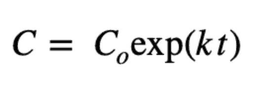
Where Co is the initial concentration.
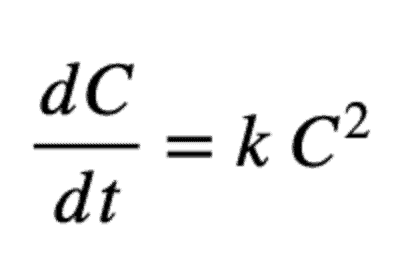
And a second-order model is:
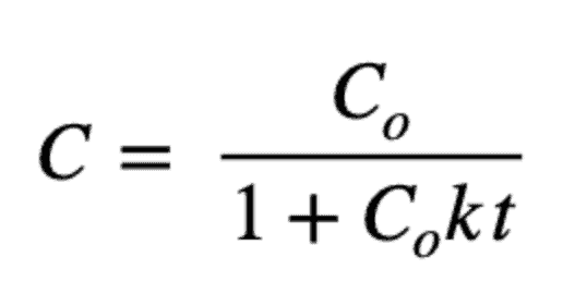
And its solution is:
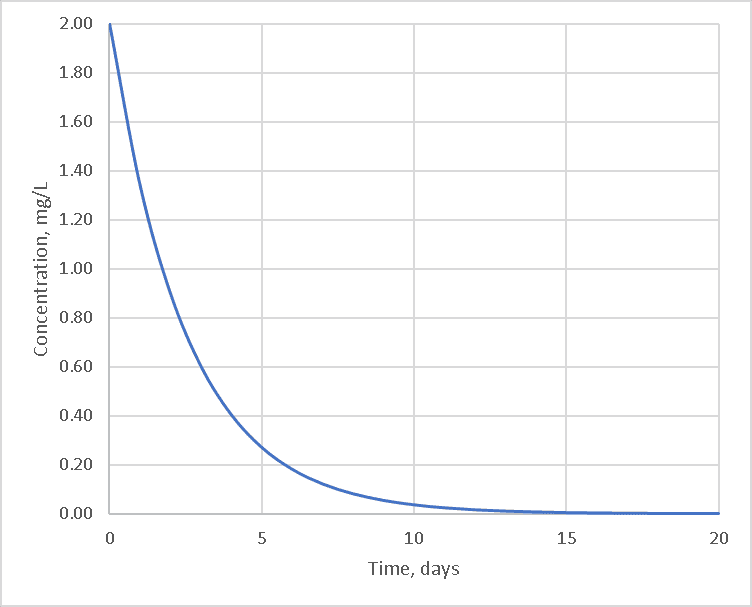
Given an initial concentration, the curve of concentration vs. time is a downward-sloping curve that tends to flatten out as the amount of chlorine available decreases.
Chlorine does not just disappear on its own, however; it must react with some other chemical. If there is only one other chemical and that chemical is present in sufficient quantity to not limit the reaction, the curve would look like the first-order solution below:
However, most waters do not contain a single chemical which reacts with the chlorine but a wide variety of chemicals that react at different rates to consume the chlorine. The most theoretically correct way to model this is to use multi-species modeling as in EPANET or WaterGEMS MSX, but this is a great deal of work in tracking down rate coefficients for each chemical as opposed to using WaterGEMS’ single effective rate constant. Those interested in calibrating an MSX chlorine model should see the blogs, “A Multi-Species Decay Model to Support Cost-Effective Chlorination in Distribution Systems,” and “Including Disinfection By-Products in a Multi-Species Decay Model to Support Cost-Effective Chlorination,” by Dr. Ian Fisher, Ph.D., an adjunct professor at the Western Sydney University Water Group in Sydney, Australia.
But most modelers would like a simple single reaction rate. Let’s take an idealized situation with three chemicals: A – which reacts very quickly with chlorine, B – which reacts somewhat slower and C – which react very slowly.
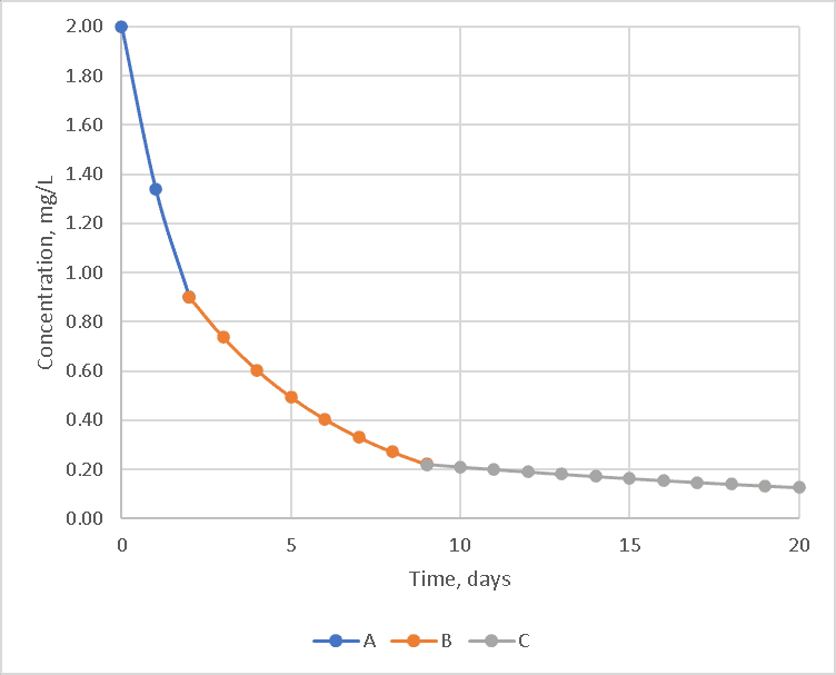
The reaction rate for the overall water can be determined in the lab by conducting a bottle, bulk chlorine decay rate where samples are collected over time and plotted. Various techniques are used to tease out the effective decay rate from real data as shown below, which may not fit a first-order rate. It is steeper initially and flatter later than a first-order solution.
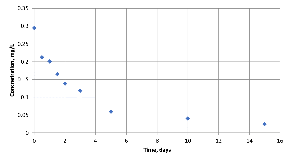
The cause of this is that the chlorine initially reacts with the fast-reacting chemical (A) until it is used up, then it reacts with other chemicals (B and then C) that react more slowly, and finally, the curve becomes much flatter as only slow reacting chemicals are left.
In the hypothetical example, this leads to three roughly first-order reactions each of which starts when the previous chemical is exhausted as shown below.
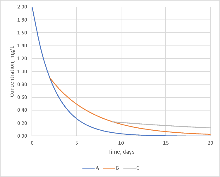
A first-order model will not fit these curves well because the reaction rate is not limited simply by the chlorine and a single reactant, but by the other chemicals. If each reaction model is calculated in series, the curve would look like the one below. The reactions with chemical A dominate for the first two days, while reactions with chemical B on days three through nine and chemical C afterward.
If there are a sufficiently diverse set of chemicals reacting with the chlorine, a single second-order curve can fit the data better than any first-order curve as shown in the graph below where the orange second-order decay line fits all three regions reasonably well. With a second-order model, it’s possible to have a single reaction rate in the WaterGEMS model.
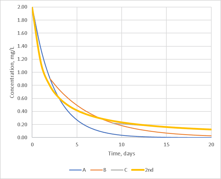
The second-order model doesn’t always work. For example, if there is a single chemical or a collection of chemicals that have similar reaction rates, the first-order model may be a very accurate prediction of concentration. If the water is very clean, such that the chemicals are exhausted before the chlorine, the graph may flatten out and reach equilibrium before getting close to zero.
In some situations, however, a single second-order bulk decay reaction may be the best solution when a modeler wants to use a single coefficient bulk decay solution.
If you want to look up past blogs, go to https://blog.bentley.com/category/hydraulics-and-hydrology/. And if you want to contact me (Tom), you can email [email protected].