2D Analysis of a Tunnel Excavation in Rock

Modeling Shotcrete and Cable Bolts: Comparison of FLAC2D and PLAXIS 2D

The 2D excavation analysis of a tunnel in a rock mass is explored in this article and some elements of comparison with an identical analysis run in FLAC2D geotechnical analysis software will be discussed. Besides a results comparison, this article will particularly focus on model construction in PLAXIS 2D geotechnical analysis software.

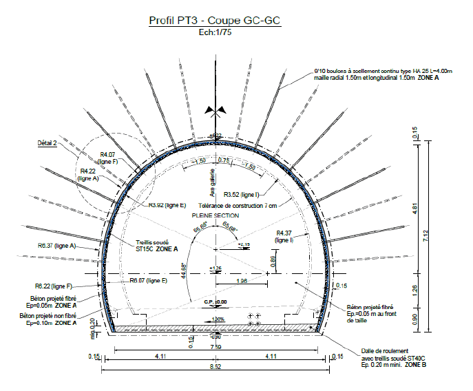
(a) Cross Section

(b) Profile

Figure 1: Tunnel drawings

Problem Description

The tunnel cross section and profile are provided in Figure 1.

The studied tunnel section is constructed at a depth of 654 m in a uniform rock mass with unit weight γ_rock = 26.7 kN.m^-3. The initial stress ratio is respectively equal to K_0,x = 0.6 (in-plane horizontal) and K_0,z = 0.8 (out-of-plane horizontal).

The tunnel is placed at an elevation of 76 m. In order to not have to physically model the entire overburden (and that would have required for the model to extend up to an elevation of 730 m vertically), a fictitious 10 m top layer with unit was introduced at an elevation of 160 m with a unit weight of γ_overb = 1522 kN.m^-3 equivalent to a 570 m thick overburden with γ_rock = 26.7 kN.m^-3 (see Figure 3).

Model Definition

Project properties are set as shown in Figure 2. The model has 80 m width and 170 m height and is using 15-noded plane strain elements.

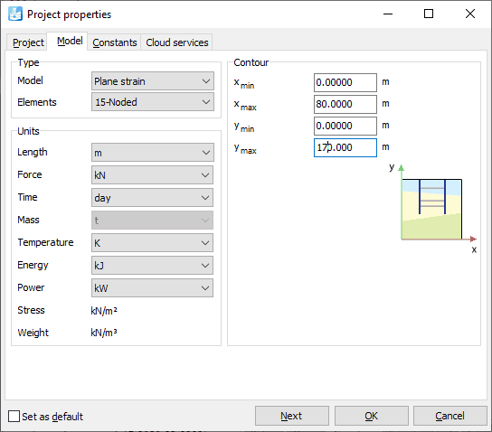
Figure 2: Project properties definition

Soil Geometry and Material Properties

One borehole is defined at x = 0 to which two distinct layers are added (see Figure 2). The soil mass is dry and the water level is set at Head = 0 m just below the considered rock mass.

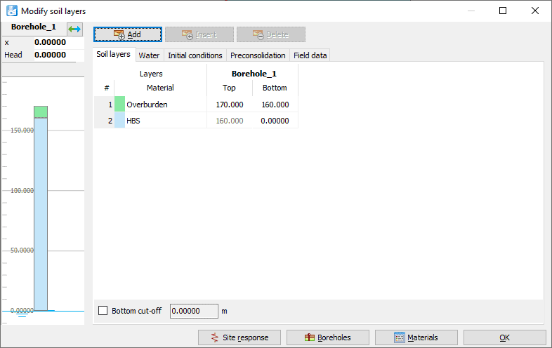
Figure 3: Soil geometry definition

The Hoek-Brown with softening (HBS) model has been used here. The main reason is the need to consider a dilatancy angle

With the classical Hoek-Brown model, the numerical solution become ill-posed when too large of a difference between the dilatancy angle

and the equivalent friction angle

is introduced. This will lead to numerical difficulties and potentially convergence toward an incorrect solution!

Although the softening behavior is not of interest here, the Hoek-Brown with softening model proposes a viscous regularization technique by the introduction of an extra parameter called the fluidity γ. The use of the viscous regularization technique in the Hoek-Brown model with softening is a definite advantage when one wants to consider a high level of non-associativity and maintained mesh-objective solution as shear plastic strains further develop.

The HBS model is therefore formulated in a visco-plasticity framework and is a stress rate-dependent model. In this context, the fluidity has only one goal in regularizing a strain localization problem, and should not introduce any significant rate effects resulting from the time-dependent variation of the boundary conditions (dynamic effect). The fluidity parameter γ must be set accordingly. A separate article explains in detail how this can be done in the framework of a simple circular tunnel excavation in rock mass. (Read to How to set up fluidity post)

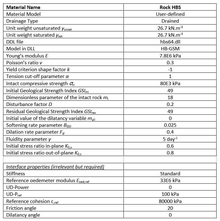
Other model parameters are summarized in Table 1. Common parameters are defined equal to those adopted in the FLAC geotechnical analysis software model. To match the assumption of a non-dilatant behavior adopted in FLAC, the initial value of the dilatancy variable m_ψi has been set to 0. Perfectly plastic behavior has also been adopted by assuming GSI_ini = GSI_res (so no softening behavior introduced here). In this context, the softening rate parameter B_GSI and dilation rate parameter F_ψ have been given arbitrary values, as they are irrelevant in the framework of a perfectly plastic behavior.

Table 1: HBS model parameter summary

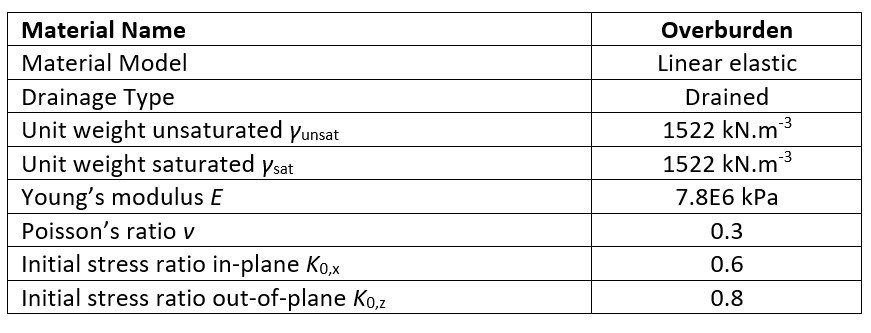
The overburden is modeled by means of a linear elastic material with identical stiffness parameters as summarized in Table 2. Initial stress ratio values are also consistent with those of the rock.

Table 2: Overburden model parameter summary

Tunnel Definition

The tunnel geometry and attached features are defined within the tunnel designer. In that respect, a tunnel is created at the reference point (x_ref = 0 m, y_ref = -76 m). Tunnel properties are defined as follows:

• Cross section mode (see Figure 4 below)
  • General tabsheet
    • Shape type: Free
    • Whole or half-tunnel : Define right half
    • Offset to begin point
      • Axis 1 = 0
      • Axis 2 = 0
  • Segments tabsheet
    • Segments[0]
      • Segment type: Line
      • Length: 3.8 m
    • Segments[1]
      • Segment type: Arc
      • Relative start angle: 68.5^o
      • Radius: 6.22 m
      • Segment angle: 44.68^o
    • Segments[2] created by extending to symmetry axis
      • Segment type: Arc [Implicit]
      • Relative start angle: 0^o [Implicit]
      • Radius: 4.06 m [Implicit]
      • Segment angle: 66.82^o [Implicit]

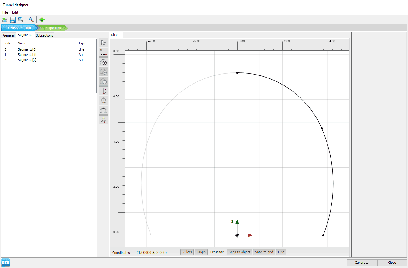
Figure 4: Tunnel cross section geometry definition

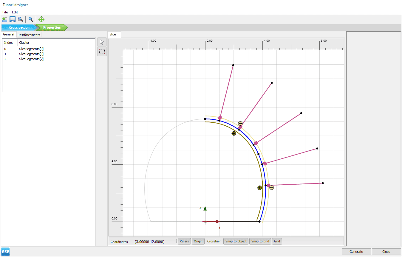
Figure 5: Tunnel segment properties definition

• Properties mode (see Figure 5 above)
  • General tabsheet
    • SliceSegments[0]:
      • Plate (defined on Segments[1])
        • Material: Shotcrete
      • Negative interface
        • Material mode: Custom
        • Material: Interface
      • SliceSegments[1]:
        • Plate (defined on Segments[2])
          • Material: Shotcrete
        • Negative interface
          • Material mode: Custom
          • Material: Interface
      • SliceSegments[2]: –
  • Reinforcement tabsheet
    • SlicePolycurveChains[0]:
      • Reversed: Active
      • Rockbolts (defined on both Segments[1] and Segments[2])
        • Material: CableBoltHA25
        • Length: 4 m
        • Breadth
          • Distribution method: Custom
          • Number: 5
          • Spacing: 1.5 m
          • Offset: 1 m

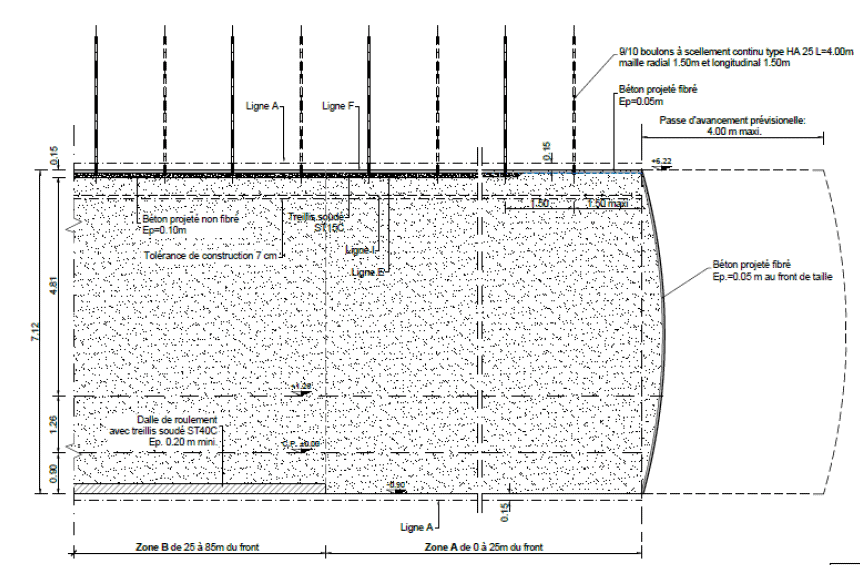
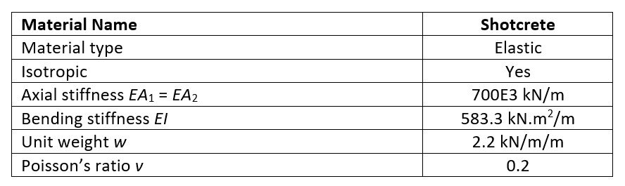
The plate is meant to represent a 10 cm shotcrete lining with properties summarized in Table 3 and has been surrounded by interface elements on both sides. The initial design considers using five 4-meter long cable bolts equally spaced every 1.5m with an initial offset of 1m from the tunnel crown. Rock bolts are modeled by means of embedded beams whose material properties are summarized in Table 5. In that respect, a companion article dealing with the modeling of rock-bolts as embedded beams in PLAXIS has been separately written.

Table 3: Summary of plate material parameters for shotcrete

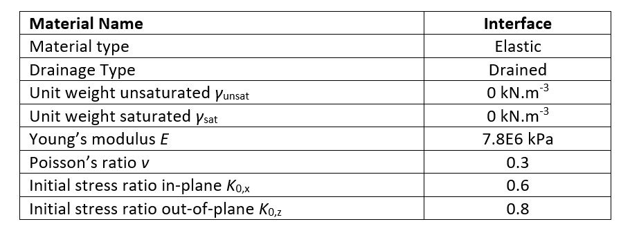
In the original FLAC calculation, the shotcrete elements have been assumed to be connected to the rock mass through perfectly elastic interface elements. The choice was made to make the same assumption in PLAXIS geotechnical analysis software. In this context, interface elements were placed between the shotcrete plate and the surrounding soil elements in the PLAXIS model. One could argue that such elastic interface elements would be the equivalent of having the plate directly connected to the soil elements. However, the two situations are not actually equivalent, because the introduction of the interface elements will also disconnect the tip of the plate to the bottom soil right underneath, avoiding the development of spurious normal force due to such a singularity (see Figure 6).

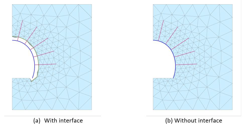
Figure 6: Shotcrete plate to rock mass connection

The assigned interface properties that were used are summarized in Table 4.

Table 4: Summary of interface material parameters for shotcrete

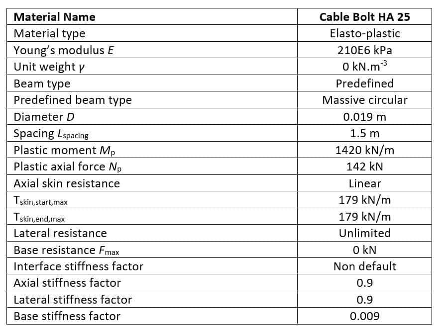
The cable bolts correspond to 19 cm diameter steel bar spaced also every 1,5 m in the out of plane direction with engineering properties given in Figure 7.

Figure 7: Tunnel cable bolt engineering parameters

Table 5: Summary of embedded beam material parameters for cable bolts

Finally, a mesh refinement box was created by adding three lines surrounding the tunnel construction area respectively:

• From (0, 70 m) to (15, 70)
• From (15, 70 m) to (15, 90)
• From (15, 90 m) to (0, 90)

The completed geometry (soil and tunnel) is finally presented in Figure 8.

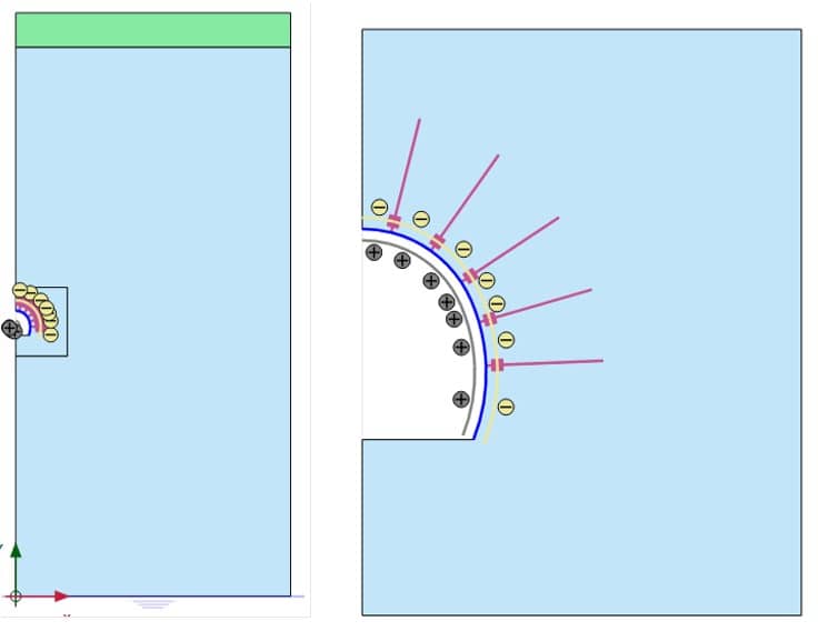
Figure 8: Overall model geometry

Mesh Generation

The mesh has been generated to provide the same node discretization as in the FLAC model. Coarseness factors of the inner tunnel clusters, plates, and cable bolts supporting lines were set to 0.1, whereas the coarseness factor of the remaining cluster inside the refinement box was set to 0.35 (see Figure 9). Mesh was generated using a Fine element distribution.

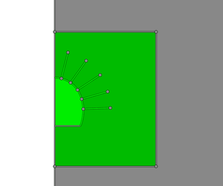
Figure 9: Mesh coarseness factor setting

Generated mesh in PLAXIS is presented in Figure 10b and is compared against grid discretization in FLAC (see Figure 10b). One should realize that FLAC was using linear elements whereas PLAXIS 2D was using fourth-order displacement elements, so even if the number of elements were considerably denser in FLAC than in PLAXIS, the number of nodes (red dots on Figure 10b) are comparable. It is an important consideration for the comparison of results that will soon follow.

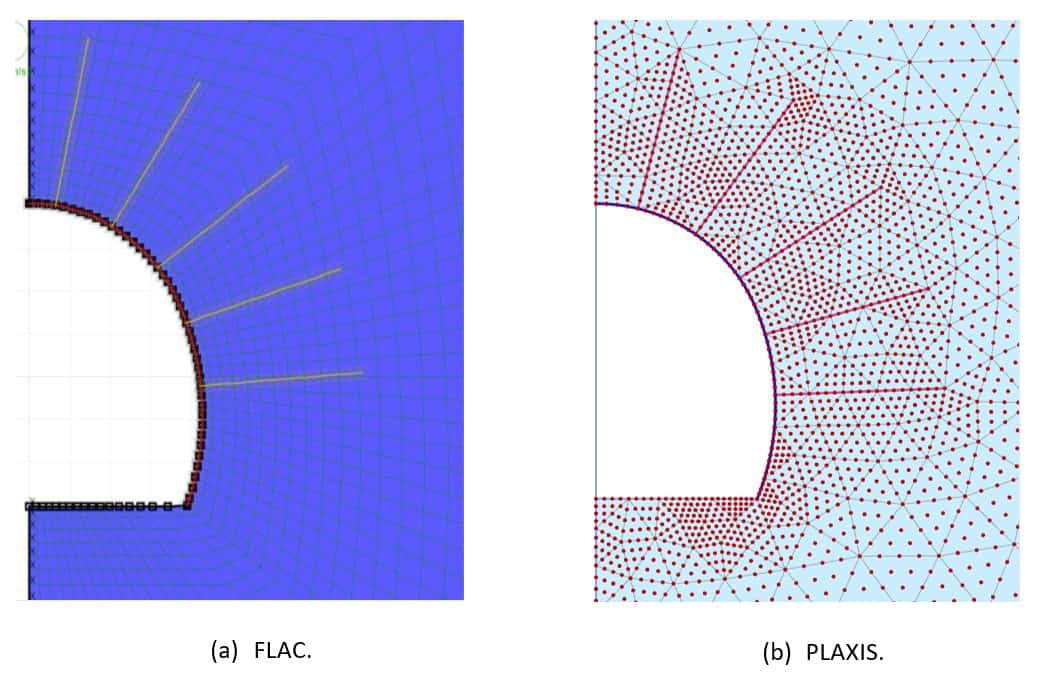
Figure 10: Mesh comparison

Construction Stage Definition

Three calculation phases are being considered:

• Initial phase (K0-procedure)
• Deconfinement 75% (Plastic analysis)
• Tunnel lining construction (Plastic analysis)

For the initial phase, there is nothing to be done to the pre-defined PLAXIS default settings.

For the deconfinement phase, the inner soil cluster must be deactivated and deconfinement (1-β) set to 75% (see Figure 11). The time interval for the phase is set to 7.5 days and the maximum load fraction per step must be set to 0.1 (enforcing at least 10 load steps for the current phase). This can be done by first unselecting the Use default iter parameters and set Max fraction per step to 0.1. For the last calculation phase, we are also advising to set arc-length control to Off, as it will lead to a faster analysis run.

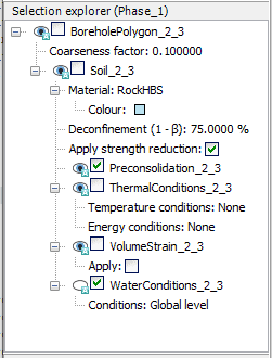
Figure 11: Soil cluster deactivation with user-defined level of deconfinement

For the final calculation phase (tunnel lining construction):

• The level of deconfinement of the previously excavated soil must be set to 100%
• All plate and embedded beam elements must be activated (from the Model Explorer, for instance)

The time interval for this last calculation phase is set to 2.5 days (10 days in total for the entire tunnel lining construction process) and the maximum load fraction per step must be set to 0.05 (enforcing at least 20 load steps for the current phase) as previously done in the phase “Deconfinement 75%.”

Finally, to properly monitor the evolution of the convergence of the excavated area, three specific mesh nodes will be chosen by selecting points for curves at:

• Tunnel crown: (0.0, 83.19)
• Tunnel invert: (0.0, 76.00)
• Tunnel left side: (4.23, 78.33)

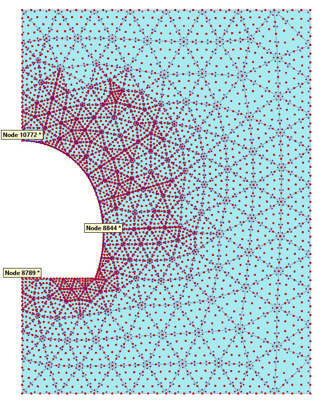
Figure 12: Curve points selection in PLAXIS Output

Results Post-processing

Displacement Contour Plots

We may first start looking at the displacement contour plot which is presented in Figure 13. Comparison against FLAC is provided where PLAXIS results have been exported to ParaView to edit the coloring mapping and set it up identical to FLAC. One can see on Figure 14 that the results are in extremely close agreement.

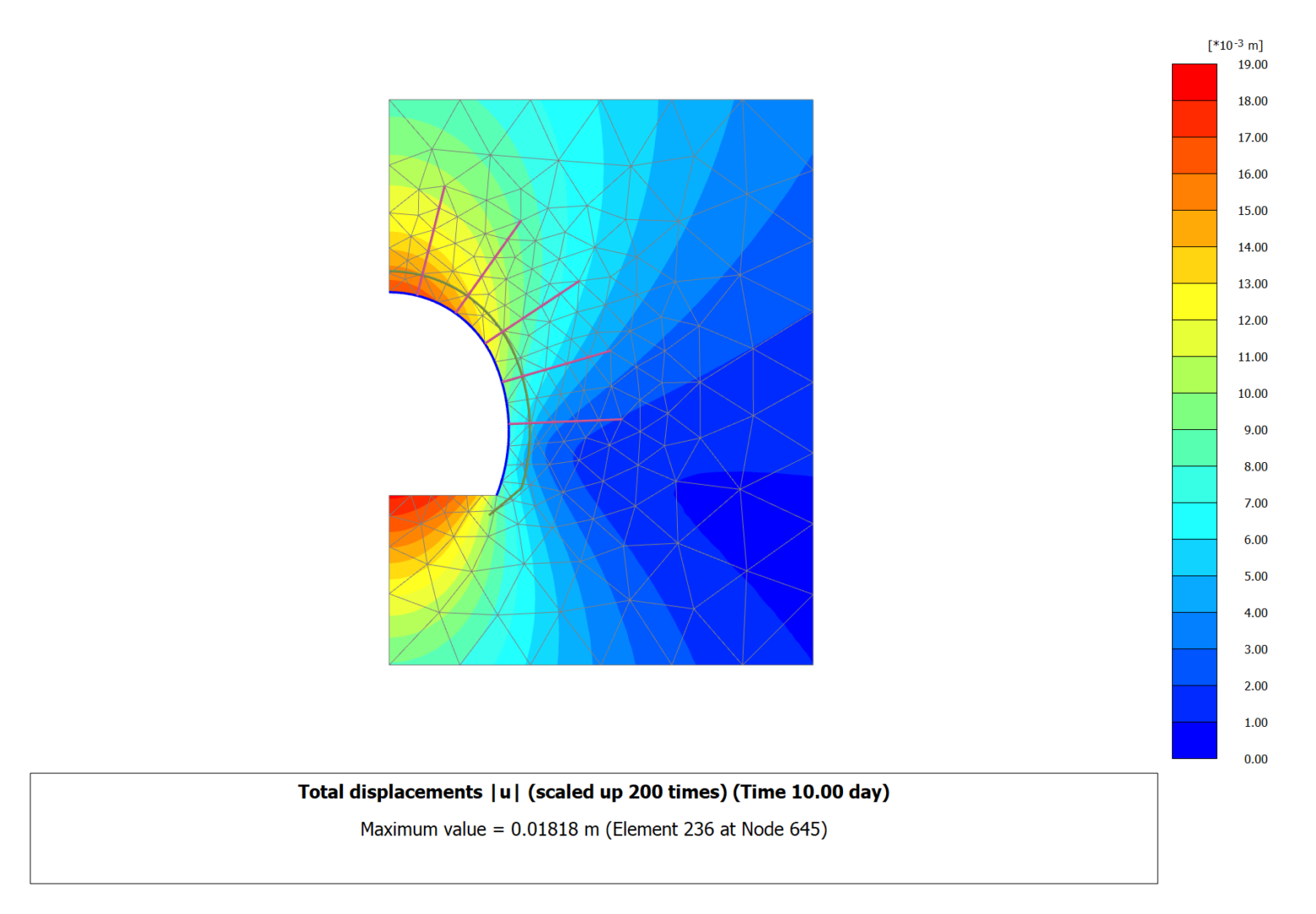
Figure 13: Contour plot of total displacement at the end of tunnel construction

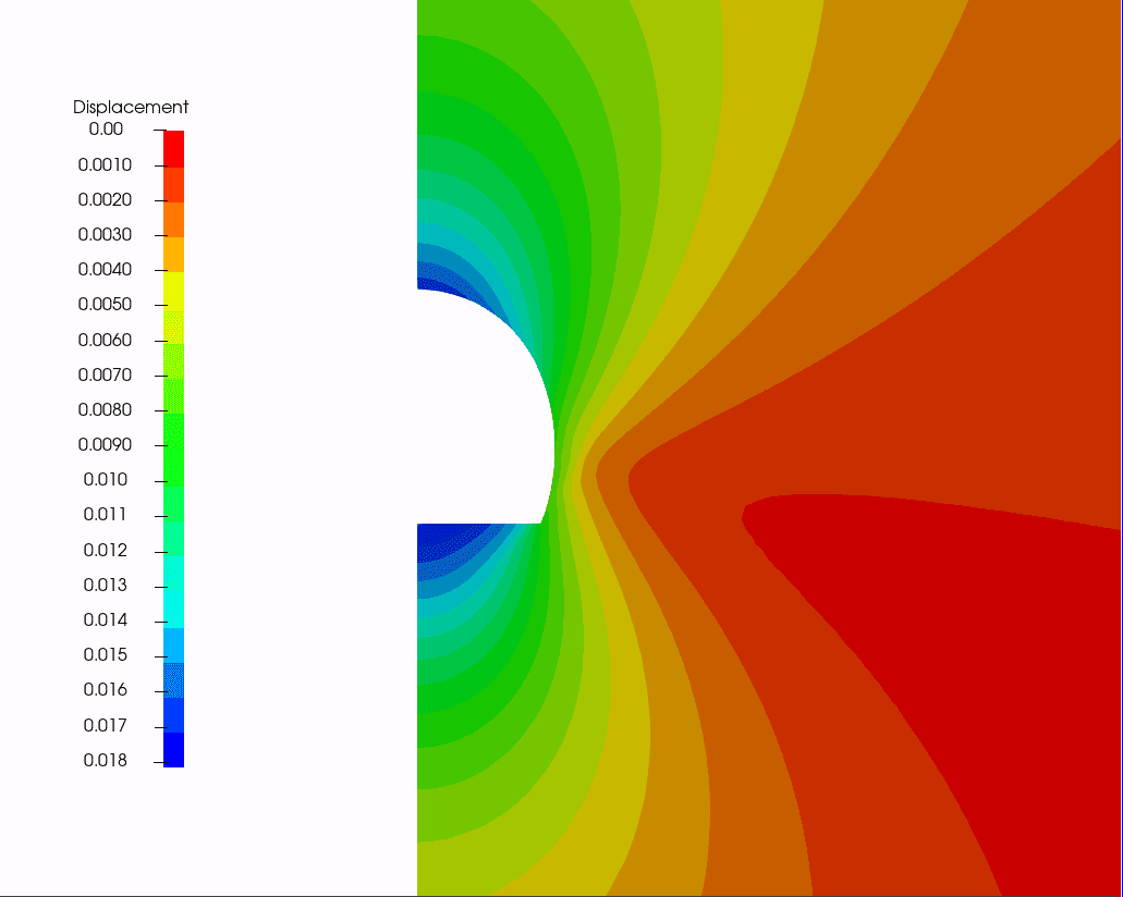
(a) PLAXIS (post-processed in ParaView)

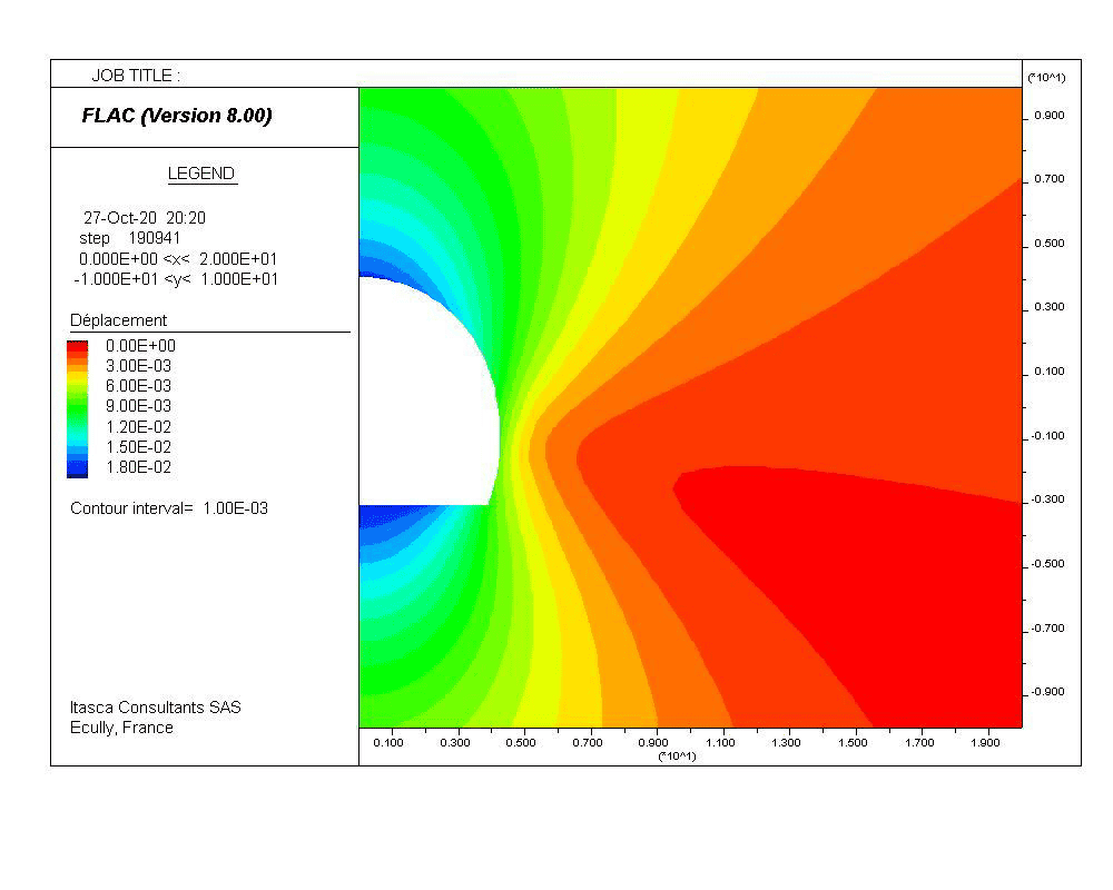
(b) FLAC

Figure 14: Comparison of total displacement contour plots at the end of tunnel construction.

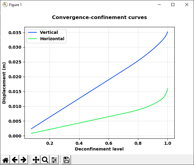
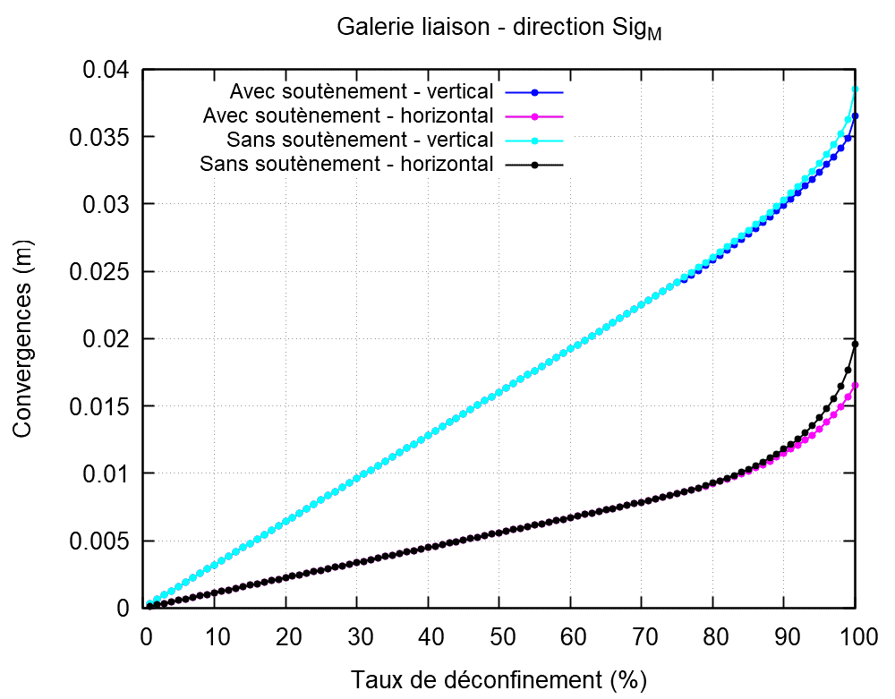
Convergence-confinement Curves

Convergence can be evaluated based on the evolution of the vertical displacement u_Y at the tunnel crown and inversion as well as the evolution of the horizontal displacement u_X on the left side. Such curves can be created though the PLAXIS Curve Manager as shown in Figure 15.

A comparison with FLAC is provided in Figure 16. The convergence-confinement curves in PLAXIS have been generated using a Python script provided in Appendix A.

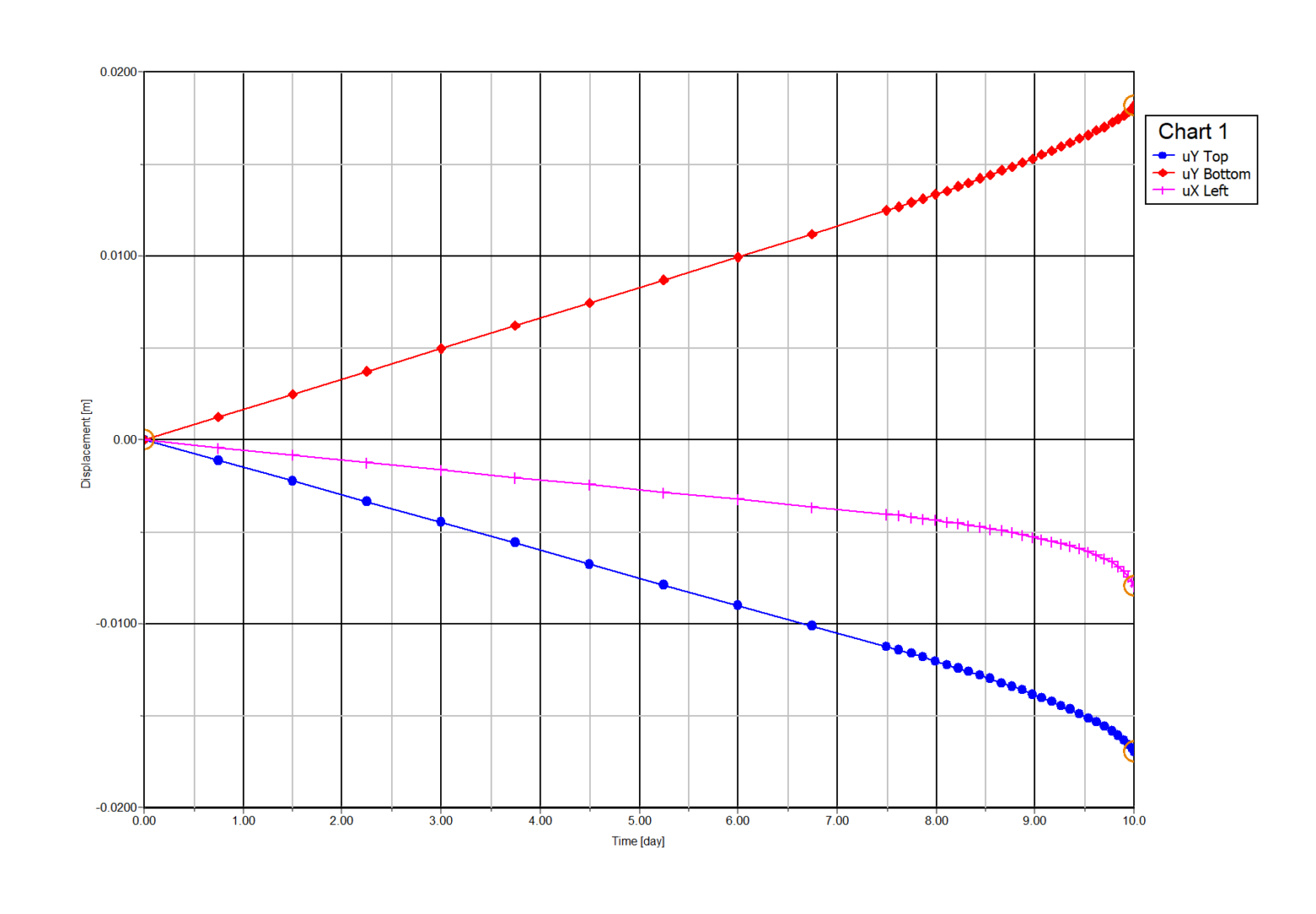
Figure 15: Displacement vs. construction time for selected points for curves

(a) PLAXIS

(b) FLAC

Figure 16: Convergence-confinement curves

Structural Forces in Shotcrete

The normal forces that develop in the shotcrete lining are displayed in Figure 17a and are compared against FLAC (see Figure 17b). Globally speaking, the results here are also in very good agreement, with a maximum force value slightly lower for PLAXIS (with N_max = 1530 kN) than for FLAC where N_max = 1660 kN (corresponding to 7.8% difference). Perhaps most important is the development of the normal force around the lowest tip of the shotcrete lining where PLAXIS provides much larger value locally than FLAC.

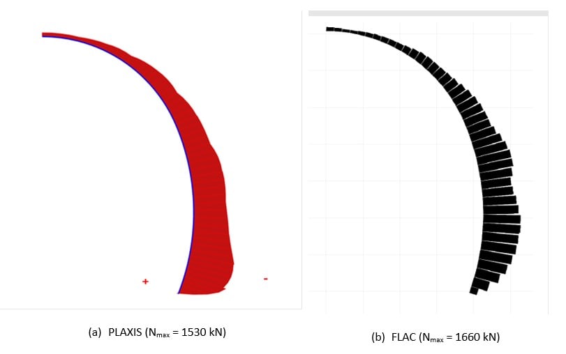
Figure 17: Normal forces in shotcrete lining plate

Axial Forces in Cable Bolt

Normal forces in cable bolts are displayed in Figure 18a and compared against FLAC (see Figure 18b). Note that the pile forces are output per meter length model and not per cable element. The axial force per cable bolt element can be retrieved by multiplying by the out-of-spacing spacing L_s = 1.5 m.

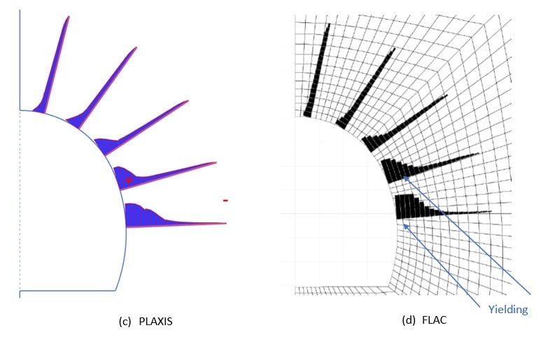
Figure 18: Normal forces in cable bolt elements

Mesh Sensitivity Analysis

This study will be concluded by a mesh sensitivity analysis. Two additional mesh configurations have been analyzed on top of the previously studied reference mesh, namely:

• Fine mesh: Obtained by setting the coarseness factor of the cluster inside the refinement box and outside the excavated cluster to 0.1 along with a Very fine element distribution.
• Very fine mesh: Obtained by setting the coarseness factor of the cluster inside the refinement box and outside the excavated cluster to 0.05 along with a Very fine element distribution.

Meshes considered for the mesh sensitivity analysis are presented in Figure 19. Results obtained in this context are presented in Figure 20 and Figure 21. These clearly show a very close agreement of results between the reference mesh and the fine mesh, along with a slight increase of both normal forces and convergences for the very fine mesh consideration (roughly 10% for the vertical confinement and 20% for the horizontal confinement).

Taking a closer look at the shear strain contour plots (see Figure 22), these clearly demonstrate the capability of the finer mesh configuration (very fine mesh) to capture the development of localized shear bands (especially at the toe of the shotcrete lining). This causes the somewhat larger horizontal convergence development as well as the local normal force spikes in the shotcrete lining at the level of the shear bands.

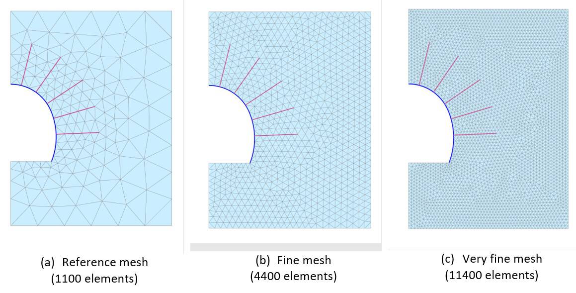
Figure 19: Mesh configuration considered for mesh sensitivity analysis

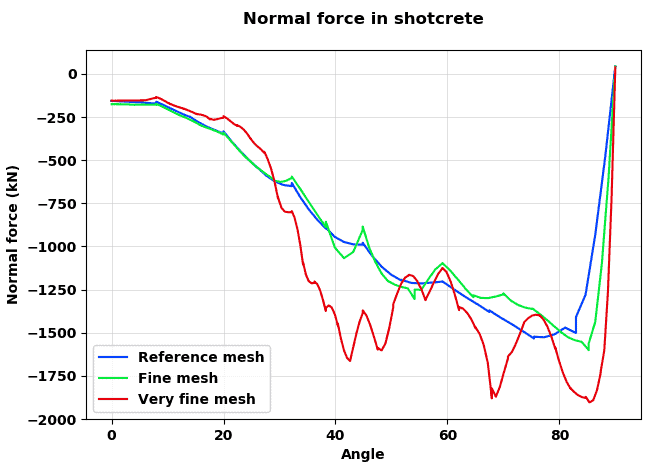
Figure 20: Normal force distribution in shotcrete lining for the different mesh refinement levels

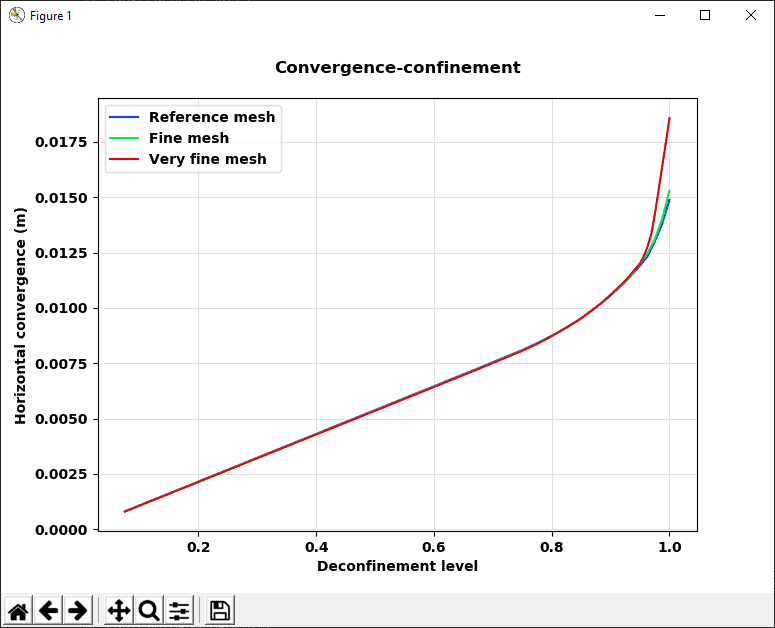
(a) Horizontal convergence

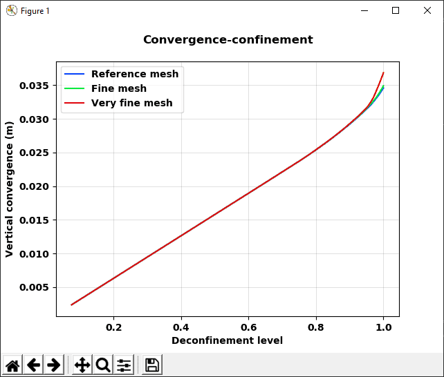
(b) Vertical convergence

Figure 21: Convergence evolution for the different mesh refinement levels.

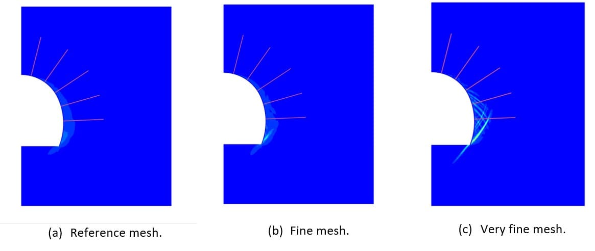
Figure 22: Plastic strain contour plots for the different mesh refinement levels.

Appendix A

Python Script for Generating the Convergence-confinement Curves

postProcessConvergence.py

from plxscripting.easy import *
import matplotlib.pyplot as plt

def gettable_time_vs_disp(phaseorder=None):

   # init data for lists
   stepids = []
   uyTop = []
   uyBot = []
   uxLeft = []
   times = []
   relTime = []

   # look into all phases, all steps:
   for phase in phaseorder:
       for step in phase.Steps.value:
           stepids.append(int(step.Name.value.replace(“Step_”, “”)))
           uyTop.append(g_o.getcurveresults(g_o.Nodes[0],
                                             step,
                                            g_o.ResultTypes.Soil.Uy))
           uyBot.append(g_o.getcurveresults(g_o.Nodes[1],
                                             step,
                                            g_o.ResultTypes.Soil.Uy))
           uxLeft.append(g_o.getcurveresults(g_o.Nodes[2],
                                             step,
                                             g_o.ResultTypes.Soil.Ux))
           # make sure step info on time is available, then add it:
           timevalue = “-“
          if hasattr(step, ‘Reached’):
               if hasattr(step.Reached, ‘Time’):
                   timevalue = step.Reached.Time.value

           times.append(timevalue)

   for time in times:
       relTime.append(time/times[-1])

   return uyTop, uyBot, uxLeft, relTime

def displayCharts(x, Y):

   plt.style.use(‘seaborn-bright’)

   plt.title(“Convergence-confinement curvesn“)
   plt.xlabel(“Deconfinement level”)
   plt.ylabel(“Displacement (m)”)
   plt.grid(b=True, which=‘major’, color=‘#666666’, linestyle=‘-‘, alpha=0.2)

   for key in Y:
       plt.plot(x, Y[key], label= key)

   leg = plt.legend()
   plt.show()

############################################################################
##########                         MAIN                        ##########
############################################################################

password = ‘9>a>LNFyt4CGvcWh’
convergenceResults = True

# Initialize output scripting server
s_o, g_o = new_server(‘localhost’, 10001, password=password)
print(‘Output reached and connected’)

if convergenceResults:
   uYTop, uYBot, uXLeft, confLevel = gettable_time_vs_disp(
       phaseorder=[g_o.Phase_1, g_o.Phase_2]
   )

   yConv = []
   xConv = []

   for uT, uB in zip(uYTop, uYBot):
      yConv.append(abs(uT – uB))

   for uL in uXLeft:
       xConv.append(abs(2 * uL))

   convPlot = {
     “Vertical”: yConv,
       “Horizontal”: xConv
   }

   displayCharts(confLevel, convPlot)