Exactly How Bad Is the Hazen-Williams Head Loss Equation for Water and Wastewater?

First of all, we need to forget about the word “exactly” in the title. When dealing with turbulent flow in water and wastewater systems, there is no theoretically perfect equation for head loss. All turbulent flow head loss equations for water are empirical to a certain extent.

If you ask university faculty who teach hydraulics, they will tell you that the Darcy-Weisbach equation is the correct equation, and they will denigrate the Hazen-Williams equation. My fluid mechanics textbook from my school days, Streeter, Fluid Mechanics, did not even mention the Hazen-Williams equation. However, if you walk down the street to the local water utility or engineering consultant office, they will be using the Hazen-Williams equation. Why the discrepancy?

There are some good reasons why the Darcy-Weisbach equation is theoretically better. It is based on a force balance between pressure and gravity forces driving the flow and the friction/turbulence restraining the flow. This equation applies to any Newtonian fluid, not just water at room temperature. It can accommodate not only a range of roughness but also a range of boundary layer types.

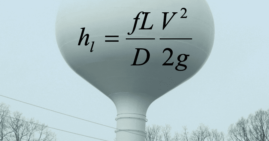
Why don’t practicing engineers use Darcy-Weisbach? Looking at the Darcy-Weisbach equation below, everyone understands the independent variables: head loss (h), length (L), diameter (D), velocity (V), gravitational acceleration (g), and some indicators of roughness (f). But when the Darcy-Weisbach equation came out, nobody could reliably determine f, the friction factor. The Darcy-Weisbach equation was developed in the mid-1800s, but whenever someone tried to measure f, it came out as a different value. What good is a constant if it isn’t a known constant?

In the meantime, two American engineers, Allen Hazen and Gardner Williams, had come up with a simpler equation where the roughness of the pipes was correlated with a single constant parameter, the Hazen-Williams C-factor, which would characterize the pipe’s roughness. This made the Hazen-Willams equation popular. Pipes designed with it worked and that’s what mattered.

There was a huge amount of research devoted to determining an equation for the friction factor in pipes. They found one in the Colebrook-White equation below. Water engineers would probably have embraced the Darcy-Weisbach equation to a greater extent, except for this messy equation needed to calculate the friction factor.

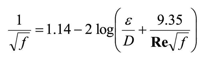
The first problem is that it can’t be solved explicitly for f because f falls on both sides of the equation. (More on this later.)

The relative size of the two terms inside the parentheses describes the mechanisms through which friction determines the head loss (and the type of turbulent flow). The first term is the relative roughness. When the first term is large, viscous forces don’t matter much and f is controlled by the roughness height (ε). (This corresponds to the top right corner of the Moody diagram where the lines are flat.) When the second term is much larger than the first, the roughness becomes negligible, and viscous forces dominate. This is the case in a very smooth pipe. When both terms are on the same order of magnitude, then both terms are important, and both roughness and viscous forces must be considered.

The Colebrook-White equation does a great job not only in calculating f, but also in understanding the nature of water flow in pipes. There are three types of turbulent flow: smooth, transition, and rough, depending on which forces predominate.

But the strength of the Colebrook-White equation is also its weakness. Accounting for the three types of flow means that 1. you can’t have a single C-factor for a pipe as in the Hazen-Williams equation, and 2. you can’t solve for f explicitly.

You could have a graphical solution, however. In the early 1940s. Louis Moody developed the Moody diagram, which could be used to graphically solve for f, given relative roughness and the Reynolds number. Before digital computers, this was the best available solution.

Once digital computers came along, the search for an explicit equation to determine C continued in earnest. It was a very common research topic in hydraulics, and everybody wanted to come up with an explicit equation that matched Colebrook-White. There were many good solutions, and the consensus winner was the Swamee-Jain equation in 1976.

So, did everyone switch to the Darcy-Weisbach equation? Not quite. The Hazen-Williams equation is so ingrained in the water industry that it is still the equation of choice for most problems. People like it and they understand the C-factor. What harm can it do?

This brings us back to the title of this blog. How different are the results between the Darcy-Weisbach equation and the Hazen-Williams equation? First, for a given pipe and liquid, there is some velocity (i.e., Reynolds number) and C-factor that gives the exact same results with either the Darcy-Weisbach equation or the Hazen-Williams equation. I’ll call that the Walski point (because I can, and I haven’t heard of a better name). This may correspond to the velocity at one point in a field or lab roughness test. As the velocity changes, the head loss calculated for the two equations begins to differ. But not by much, especially for a smooth or transition flow. For rough pipes (and actually rough boundary layer), as the velocity changes, the results for the two equations differ more and more. But by how much?

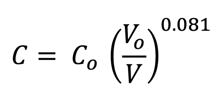
Years ago, I looked at the worst-case differences and came up with this simple equation to adjust C-factors based on velocity. If you measured C (Co) at one velocity (Vo) and wanted to apply it to a different velocity, you could adjust C using the equation.

For derivation, see Walski (1984).

Let’s take an example where the measured C-factor is 80 at 2 ft/s and you want to know C at 10 ft/s. The new C-factor would be 70 at 10 ft/s. This is an extreme case because you would more likely measure C at 5 ft/s and want to know C at 8 ft/s. In that case, it would be 77. These differences are not huge, but they show that C-factors for fully rough flow should not be extrapolated too far from the velocity where they were measured. In most cases, the differences between the two values would be small and within the error in measurement of C.

How much difference does it make in a realistic rough pipe? I set up an example problem in FlowMaster with these characteristics.

Q = 400 gpm
V = 2.5 ft/s
D = 8 in.
L = 500 ft
ε = 0.0162 ft
f = 0.056
h loss = 4 ft

Working back from this data, the C-factor is 81.

Now let’s double the flow. Here are the changes:

Q = 800 gpm
V = 5 ft/s
f = 0.053
h loss = 16 ft

The roughness height stayed the same. To achieve the same head loss, the C-factor is now 77, using either FlowMaster or the 0.081 equation.

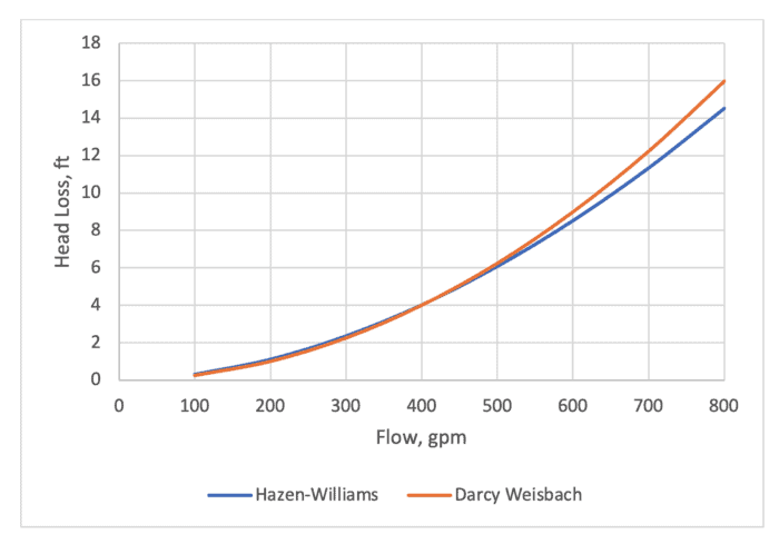
Looking at this graphically, you can see that the differences for this pipe are only visible at high velocity (flow) and the differences in head loss are not very large.

What action should you take? As long as you are not in the situation where you measured C in rough flow at a low velocity and are now applying it at a much higher velocity, the results should be the same whether you use Darcy-Weisbach or Hazen-Williams. If not, you may want to lower the C-factor using the equation above, but the differences in results will be small in most cases. In general C-factor tests are run at a fairly high velocity.

As I asked in the title, is the Hazen-Williams equation all that bad? No, it works, but you should understand the potential limitations.

Swamee, P.K. and Jain, A.K., 1976, “Explicit Equation for Pipe Flow Problems,” ASCE Hydraulic Division, 102:HY5, p. 657.

Walski, T., 1984, Analysis of Water Distribution Systems, Van Nostrand Reinhold, New York.

If you want to look up past blogs, go to https://blog.bentley.com/category/hydraulics-and-hydrology/.  And if you want to contact me (Tom), you can email tom.walski@bentley.com.

Want to learn more from our resident water and wastewater expert? Join the Dr. Tom Walski Newsletter today!