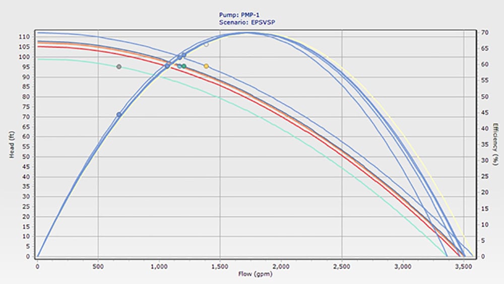
“You have a pump that’s capable of 70% efficiency running at 63%, 60%, and even 45% efficiency as flows vary over the course of a day,” Dan said. “Note those points on the curves.”
“Now let’s look at how the original constant speed pump would do,” Dan said as he switched scenarios. Up came another display.
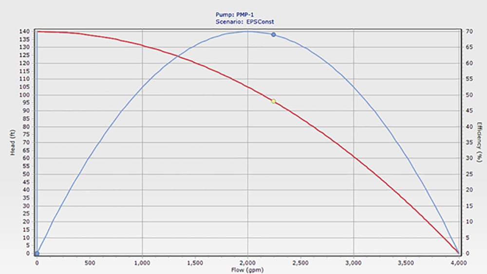
“The constant speed pump runs at the same efficient speed with an efficiency of around 69%, and it turns off when its job is done. The most cost-effective speed to run a pump is ‘Off.’ If you buy the right pump for the system, when it is on, it’ll be running efficiently,” Dan said.
Jim sheepishly asked, “How does this look over the course of the day?”
Dan pulled up another set of graphs. “Time series graphs are easy,” he said. “Just pick the pump and the parameter you want to graph. In our case, we’ll look at three parameters: the relative speed—that’s actual speed divided by full speed; wire-to-water efficiency from the electrical power entering the motor to the water; and cost per million gallons pumped. Here’s your answer.”
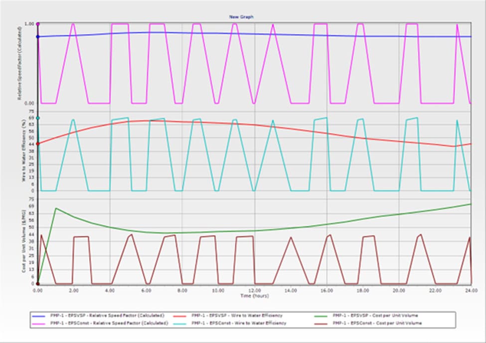
“A picture is worth a thousand words,” Dan said. “In the top graph, the blue line shows changes of speed with the VFD. The magenta line shows when the constant speed pump is off or on. The middle graph shows that the constant speed pump, the cyan-colored line, is more efficient when it’s on than the variable speed pump, the red line. But the constant pump isn’t always on like the variable speed pump. The bottom line is clear: The cost to run the constant speed pump is lower than the variable speed pump over the entire day.”
Jim asked, “Can I just find a cost summary for a given scenario?”
Dan smiled. “Just hit the summary tab,” he said.
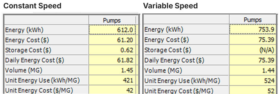
Dan did some quick math to calculate the annual cost difference: (75.39 – 62.82) x 365. “That means saving $4,588 per year with constant speed pumping. Plus, we wouldn’t need to buy a VFD,” Dan said. “Last I heard, they aren’t giving those away for free.”
“So, I should never use a variable speed pump?” Jim asked.
Dan grimaced. “No, there are a lot of situations where variable speed pumping is valuable. The point is that you need to analyze the life cycle energy costs of the pumps when you are selecting them. OpenFlows Water does the hard work for you.
“And this one run we did for average day flows shouldn’t be the end of the analysis,” Dan added. “You should make some runs for max days, different days of the week, or future year flows. In the old days, I had to do these calculations by hand, and I needed to make a number of simplifying assumptions. But with Bentley’s scenario management, you can accurately crank out all the runs you need in no time.”
Jim chimed in. “I guess that’s all I need to know about VFDs and pumps?”
“No, you’re just starting out,” Dan said, smiling. “Have you heard about the ‘parasitic energy demand’ of a VFD? VFDs take the sine wave of electricity and break it into little pieces, then reassemble it into a sine wave at the frequency you want. It’s pretty amazing technology. But no device is perfectly efficient. Some energy is lost along the way. At full speed, the VFD doesn’t lose much energy. But as the speed slows down, the parasitic demand increases. If you don’t believe me, stand next to a VFD when it’s running. You’ll feel the waste as heat energy coming off.”
Jim looked down at his shoes. “I have a lot to learn. Sorry to have taken up your time.”
Dan grinned. “This was a teachable moment, and we both benefited from it. Let me get you a cup of coffee from the breakroom. I’ll tell you some stories about pumps I’ve known and loved.”
Jim replied with a smile, “I’d love to hear your stories, but I’ll pass on the breakroom coffee. It tastes like activated sludge.”
Jim raised his eyebrows: “How would you know how activated sludge tastes?”