Most hydraulic engineers would admit that the Darcy-Weisbach equation is the most theoretically correct equation for head loss in pipe flow. It is based on a force balance between the driving forces of pressure and gravity, offset by head loss and can be applied to any Newtonian fluid. It’s pretty elegant looking.

Where h = head loss, L = pipe length, D = diameter, V = velocity, g = gravitational acceleration and don’t forget about f, the mysterious friction factor.
The Darcy-Weisbach equation was developed around 1850, but it took decades of research before engineers could determine how to determine f. It would have been great if f was a nice constant like 3.1416. But f varied based on all sorts of things like pipe roughness, velocity, fluid density, and viscosity… f is anything but constant.
Ludwig Prandtl and his students in Germany did the most noteworthy research. The most famous experiments were conducted by Johan Nikuradse, who glued uniform sand grains inside pipes, measured f and tried to correlate those measurements with f. They found that f correlated with the Reynolds number (ratio of inertial and viscous forces) and pipe relative roughness.
Here is where Cyril Colebrook and Cedric White, see the title, finally come in. In the 1930s, they derived the most widely accepted equation to determine f. Unfortunately, the equation is not pretty. It is actually quite ugly.
Where e = equivalent sand grain roughness, R = Reynold number
Yuck. There are some bad things about this equation. The worst part is that you can’t solve it explicitly for f. Notice that f is on both sides of the equation. So, you need to guess a value and keep iterating until you converge to f. Remember that this was back in the days when calculations were done with slide rules. You can understand why engineers preferred to use the Hazen Williams equation with all its imperfections (limited range of application, water only, strange exponents).
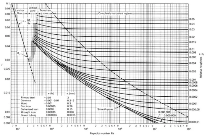
To get around some of the issues with the Colebrook-White equation, in the 1940s, Lewis Moody, a professor at Princeton Univ., came up with a graphical solution (the famous, or infamous, Moody Diagram) that reduces the effort involved with relating head loss to flow. Until computers came along, it was the method of choice for those insisting on using the Darcy-Weisbach equation. It isn’t very pretty, either.
Moody Diagram
Since then, dozens of researchers have been publishing papers with an explicit solution to the Colebrook-White equation. That is, and equation you can write as
f = …
I must confess that I was a co-author on one of those papers. We could approximate the Colebrook-White equation to something like six significant figures. Stop and think about how silly that is. The Colebrook-White equation is only accurate to about two significant figures, and any digits after that are essentially numerical noise.
The approximation we use in OpenFlows WaterGEMS and OpenFlows WaterCAD is the Swamee-Jain equation, which is one of the most widely used. It’s almost as ugly as the Colebrook-White equation, but it solves a good bit faster because you don’t need to iterate.
While the Colebrook-White equation is held up as the gold standard in friction factor methods, does it really deserve such a position of honor? It uses only one parameter, roughness height, to characterize roughness. But doesn’t roughness shape and spacing also matter? It does, and there are other equations and diagrams for different shapes and spacing. There are actually multiple different regimes of turbulent flow. Some of these include isolated roughness elements, hyperturbulent (wake interference), and quasi-smooth flow, each with its own approach to determining a friction factor. Many have the same basic shape as the Moody diagram, with Reynolds number on the horizontal axis and friction factor on the vertical, but the curves are very different. (A good reference if you want to follow up is Morris and Wiggert’s book, Applied Hydraulics in Engineering.)
Remember that the Colebrook-White equation is still an empirical equation. You can’t derive it from F = ma, and it doesn’t even fit Nikuradse’s original data very well. But the equation has served us well over the years. We need to remember that it is still an empirical equation and has its limitations.
Want to learn more from our resident water and wastewater expert?
Join the Dr. Tom Walski Newsletter today!


